If you’ve ever used ggplot2 to create figures for a journal article, you’ve probably experienced this: your plot looks perfect in RStudio, but when you save it at the required dimensions (e.g. relative to an A4 page), the proportions look completely off (e.g. lines too thin/big, the font doesn’t look right). I used to spend hours tweaking each plot individually, trial after trial, until it finally looks acceptable. This is nightmare especially if you want to update figures after changing something in the analysis.
This guide walks through my workflow for creating figures that are actually publication-ready, without writing custom code for every plot or endlessly fiddling with parameters. The goal is to spend less time adjusting figures.
Journal requirements: start with the right dimensions
Before you even start plotting, check your target journal’s figure guidelines. Common width limits range from 177.8 mm to 200 mm (e.g., Elsevier, Science, Cell). The width is usually the constraining factor, so design with that in mind.
Useful resources:
Here’s a typical scenario: you create a multi-panel figure in RStudio, set fig.width and fig.height in inches and everything looks fine. But when you save it at the required millimeter dimensions, the result is disappointing.
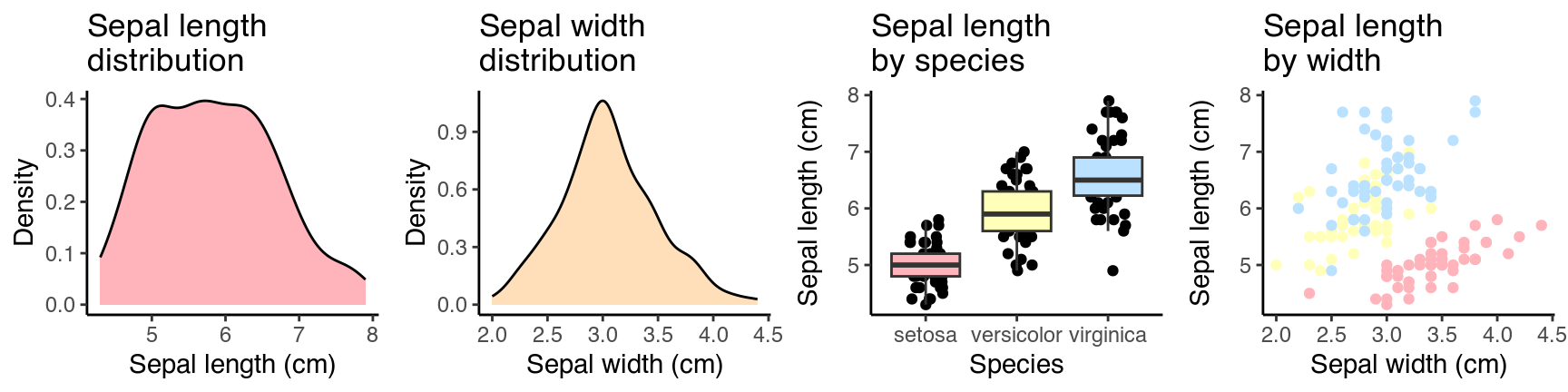
Let’s illustrate with an example—a 1×4 panel figure using the classic iris dataset. Settings used for the chunk: fig.width = 9, fig.height = 2.25.
In my mind, the results looks pretty decent (e.g. font & geom sizes) even without any further styling.
 1
 2
 3
 4
 5
 6
 7
 8
 9
10
11
12
13
14
15
16
17
18
19
20
21
22
23
24
25
26
27
28
29
30
|
# Colours
colour_pal <- c("#ffb3ba", "#ffdfba", "#ffffba", "#baffc9", "#bae1ff")

p1 <- ggplot(iris, aes(x = Sepal.Length)) +
  geom_density(fill = colour_pal[1]) +
  theme_classic() +
  labs(x = "Sepal length (cm)", y = "Density", title = "Sepal length\ndistribution")

p2 <- ggplot(iris, aes(x = Sepal.Width)) +
  geom_density(fill = colour_pal[2]) +
  theme_classic() +
  labs(x = "Sepal width (cm)", y = "Density", title = "Sepal width\ndistribution")

p3 <- ggplot(iris, aes(x = Species, y = Sepal.Length, fill = Species)) +
  geom_jitter(height = 0, width = 0.2) +
  geom_boxplot(outlier.shape = NA) +
  theme_classic() +
  scale_fill_manual(values = colour_pal[c(1, 3, 5)]) +
  theme(legend.position = "none") +
  labs(x = "Species", y = "Sepal length (cm)", title = "Sepal length\nby species")

p4 <- ggplot(iris, aes(x = Sepal.Width, y = Sepal.Length, colour = Species)) +
  geom_point() +
  theme_classic() +
  scale_colour_manual(values = colour_pal[c(1, 3, 5)]) +
  theme(legend.position = "none") +
  labs(x = "Sepal width (cm)", y = "Sepal length (cm)", title = "Sepal length\nby width")

# Combine the figures using cowplot
plot_grid(p1, p2, p3, p4, nrow = 1, ncol = 4, align = "hv")
|
Now, save it as a 180 mm wide figure:
 1
 2
 3
 4
 5
 6
 7
 8
 9
10
11
12
13
14
15
|
# Combine the figures using cowplot and save as an object
p <- plot_grid(p1, p2, p3, p4, nrow = 1, ncol = 4, align = "hv")

# Get the r-chunk ratio
fig_ratio <- 2.25/9

# Create folder to save figures in
dir.create("pub_fig_guide", showWarnings = FALSE)

# Save to file
ggsave(p, filename = "pub_fig_guide/fig1.png",
       dpi = 1000,
       width = 180,
       height = 180*fig_ratio,
       units = "mm")
|
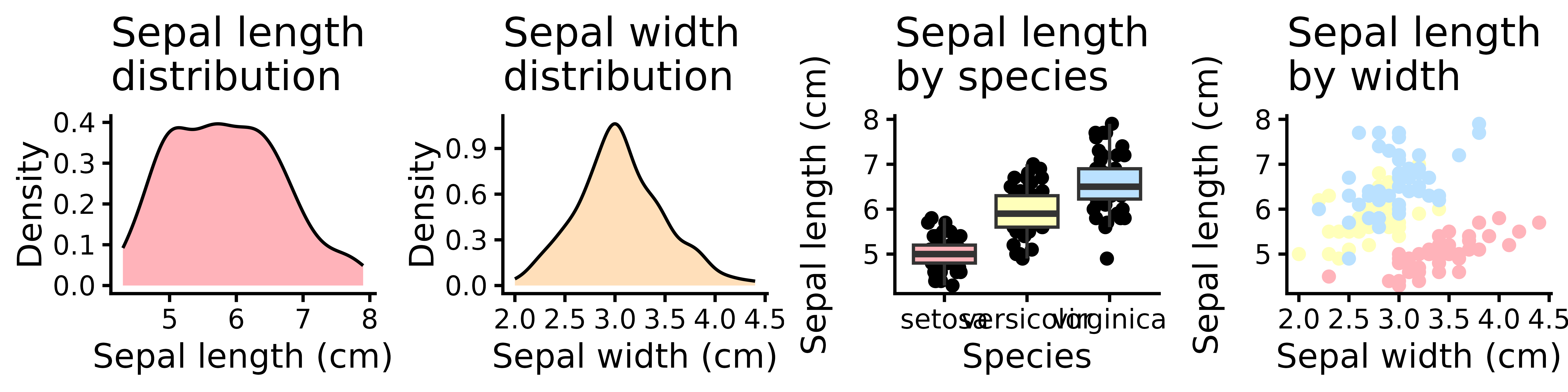
Some elements look okay, but many are out of proportion. So, here is how I deal with this.
My current approach: A custom theme and updated defaults
1. Create a custom theme function
Instead of adjusting each plot’s theme individually, I define a reusable theme_journal() function. It standardizes text sizes, line widths and other elements based on a chosen base theme but you can go much further with this, which I won’t cover.
 1
 2
 3
 4
 5
 6
 7
 8
 9
10
11
12
13
14
15
16
17
18
19
20
21
22
23
24
25
26
27
28
29
30
31
32
33
34
35
36
37
|
theme_journal <- function(base_size = 7, linewidth = 0.35, theme_name = "classic") {
  # Select a base theme from https://ggplot2.tidyverse.org/reference/ggtheme.html
  if(theme_name == "grey" | theme_name == "gray"){
    base_theme <- theme_grey(base_size = base_size)

  } else if(theme_name == "bw"){
    base_theme <- theme_bw(base_size = base_size)

  } else if(theme_name == "linedraw"){
    base_theme <- theme_linedraw(base_size = base_size)

  } else if(theme_name == "light"){
    base_theme <- theme_light(base_size = base_size)

  } else if(theme_name == "dark"){
    base_theme <- theme_dark(base_size = base_size)

  } else if(theme_name == "minimal"){
    base_theme <- theme_minimal(base_size = base_size)

  } else if(theme_name == "classic"){
    base_theme <- theme_classic(base_size = base_size)

  } else {
    stop("Unknown theme. Check https://ggplot2.tidyverse.org/reference/ggtheme.html")
  }

  # Base them plus customisation
  base_theme +
    theme(text = element_text(color = "black", size = base_size),
          axis.text = element_text(size = base_size * 0.9),  # 90% of base
          axis.line = element_line(linewidth = linewidth),
          axis.ticks = element_line(linewidth = linewidth),
          legend.text = element_text(size = base_size * 0.9), # 90% of base
          legend.key.size = unit(0.5, "lines"),
          plot.title = element_text(hjust = 0.5, size = base_size))
}
|
2. Update default aesthetics for geoms
To do this, you also have to know the default values but finding the default aesthetic values for each geom can be annoying. Fortunately, you can inspect them directly (e.g., GeomPoint$default_aes) and then set new defaults globally using update_geom_defaults().
1
2
3
4
|
# Can be checked via GeomDensity$default_aes, GeomBoxplot$default_aes etc.
update_geom_defaults("point", list(size = 0.5))
update_geom_defaults("density", list(linewidth = 0.25))
update_geom_defaults("boxplot", list(linewidth = 0.25))
|
This way, every subsequent plot uses these updated defaults - no need to manually set size or linewidth in each geom_*() call.
Now, let’s rebuild the same four-panel figure using our custom theme and updated defaults:
 1
 2
 3
 4
 5
 6
 7
 8
 9
10
11
12
13
14
15
16
17
18
19
20
21
22
23
24
25
26
27
28
29
30
31
32
33
34
|
p1 <- ggplot(iris, aes(x = Sepal.Length)) +
  geom_density(fill = colour_pal[1]) +
  theme_journal() +
  labs(x = "Sepal length (cm)", y = "Density", title = "Sepal length\ndistribution")

p2 <- ggplot(iris, aes(x = Sepal.Width)) +
  geom_density(fill = colour_pal[2]) +
  theme_journal() +
  labs(x = "Sepal width (cm)", y = "Density", title = "Sepal width\ndistribution")

p3 <- ggplot(iris, aes(x = Species, y = Sepal.Length, fill = Species)) +
  geom_jitter(height = 0, width = 0.2) +
  geom_boxplot(outlier.shape = NA) +
  theme_journal() +
  scale_fill_manual(values = colour_pal[c(1, 3, 5)]) +
  theme(legend.position = "none") +
  labs(x = "Species", y = "Sepal length (cm)", title = "Sepal length\nby species")

p4 <- ggplot(iris, aes(x = Sepal.Width, y = Sepal.Length, colour = Species)) +
  geom_point() +
  theme_journal() +
  scale_colour_manual(values = colour_pal[c(1, 3, 5)]) +
  theme(legend.position = "none") +
  labs(x = "Sepal width (cm)", y = "Sepal length (cm)", title = "Sepal length\nby width")

# Combine the figures using cowplot and save as an object
p <- plot_grid(p1, p2, p3, p4, nrow = 1, ncol = 4, align = "hv")

# Save to file
ggsave(p, filename = "pub_fig_guide/fig2.png",
       dpi = 1000,
       width = 180,
       height = 180*fig_ratio,
       units = "mm")
|
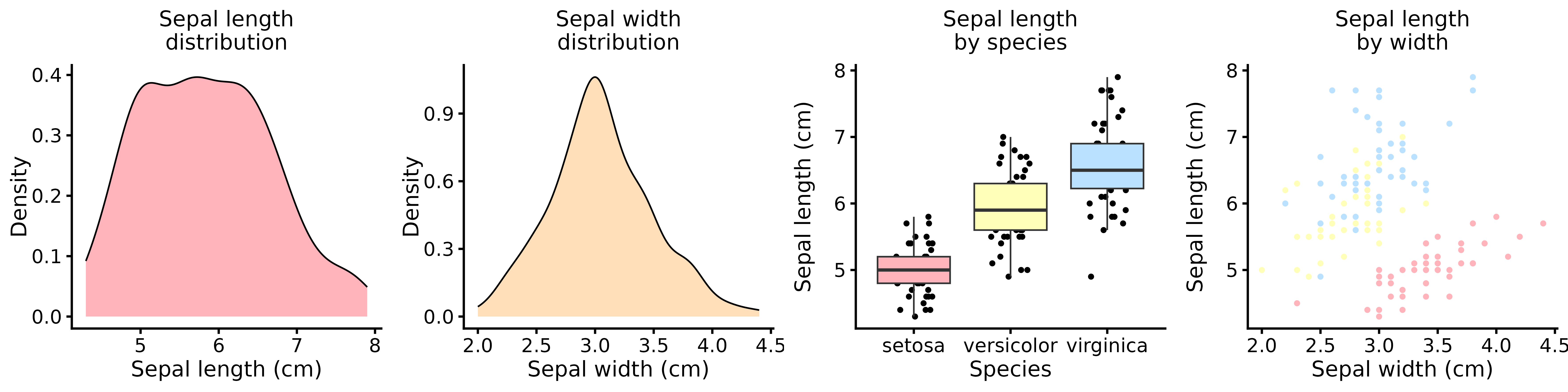
The result is a clean, proportionally balanced figure that meets typical journal requirements with minimal manual adjustment.
For greater flexibility, consider exporting your figures as SVG instead of PNG. SVG files are:
- Scalable without quality loss.
- Editable in vector graphics software like Inkscape.
- Version-control friendly (text-based).
Use svglite for reliable SVG export:
1
2
3
4
5
6
|
# Use this because viewport/scaling issues
library(svglite)
ggsave(p, filename = plot_filename,
       device = svglite,  width = 90,
       height = 45,  units = "mm",
       scaling = 1,  fix_text_size = FALSE)
|
When importing into Inkscape, select the option “Include SVG image as editable object(s) in the current file.” When I exported my .svg files without svglite, the figures have very odd artefacts in them.
Additional tips
- PowerPoint users: You can convert SVG images into editable PowerPoint objects.
- Preview tools: Check out
ggview::canvas() to set your RStudio viewing pane to match export proportions and ggpreview() from the nflplotr package for quick previews.
Final thoughts
Creating publication-ready figures in R doesn’t have to be a painful process of trial and error. By defining a custom theme, updating geom defaults globally, and choosing the right export format, you can produce consistent, journal-compliant figures with minimal repetitive code.
Session details
Click here for detailed for libraries used and session information.
1
|
sessioninfo::session_info()
|
 1
 2
 3
 4
 5
 6
 7
 8
 9
10
11
12
13
14
15
16
17
18
19
20
21
22
23
24
25
26
27
28
29
30
31
32
33
34
35
36
37
38
39
40
41
42
43
44
45
46
47
48
49
50
51
52
53
54
55
56
57
58
59
60
61
|
## ─ Session info ───────────────────────────────────────────────────────────────
##  setting  value
##  version  R version 4.4.0 (2024-04-24)
##  os       Ubuntu 22.04.5 LTS
##  system   x86_64, linux-gnu
##  ui       X11
##  language en_GB:en
##  collate  en_GB.UTF-8
##  ctype    en_GB.UTF-8
##  tz       Asia/Shanghai
##  date     2026-02-05
##  pandoc   3.1.1 @ /usr/lib/rstudio/resources/app/bin/quarto/bin/tools/ (via rmarkdown)
##
## ─ Packages ───────────────────────────────────────────────────────────────────
##  package     * version date (UTC) lib source
##  bslib         0.7.0   2024-03-29 [1] CRAN (R 4.4.0)
##  cachem        1.1.0   2024-05-16 [1] CRAN (R 4.4.0)
##  cli           3.6.2   2023-12-11 [1] CRAN (R 4.4.0)
##  colorspace    2.1-0   2023-01-23 [1] CRAN (R 4.4.0)
##  cowplot     * 1.1.3   2024-01-22 [1] CRAN (R 4.4.0)
##  digest        0.6.35  2024-03-11 [1] CRAN (R 4.4.0)
##  dplyr         1.1.4   2023-11-17 [1] CRAN (R 4.4.0)
##  evaluate      0.23    2023-11-01 [1] CRAN (R 4.4.0)
##  fansi         1.0.6   2023-12-08 [1] CRAN (R 4.4.0)
##  fastmap       1.2.0   2024-05-15 [1] CRAN (R 4.4.0)
##  generics      0.1.3   2022-07-05 [1] CRAN (R 4.4.0)
##  ggplot2     * 3.5.2   2025-04-09 [1] CRAN (R 4.4.0)
##  glue          1.7.0   2024-01-09 [1] CRAN (R 4.4.0)
##  gtable        0.3.5   2024-04-22 [1] CRAN (R 4.4.0)
##  htmltools     0.5.8.1 2024-04-04 [1] CRAN (R 4.4.0)
##  jquerylib     0.1.4   2021-04-26 [1] CRAN (R 4.4.0)
##  jsonlite      1.8.8   2023-12-04 [1] CRAN (R 4.4.0)
##  knitr         1.50    2025-03-16 [1] CRAN (R 4.4.0)
##  lifecycle     1.0.4   2023-11-07 [1] CRAN (R 4.4.0)
##  magrittr      2.0.3   2022-03-30 [1] CRAN (R 4.4.0)
##  munsell       0.5.1   2024-04-01 [1] CRAN (R 4.4.0)
##  pillar        1.9.0   2023-03-22 [1] CRAN (R 4.4.0)
##  pkgconfig     2.0.3   2019-09-22 [1] CRAN (R 4.4.0)
##  plyr        * 1.8.9   2023-10-02 [1] CRAN (R 4.4.0)
##  R6            2.5.1   2021-08-19 [1] CRAN (R 4.4.0)
##  Rcpp          1.0.12  2024-01-09 [1] CRAN (R 4.4.0)
##  rlang         1.1.4   2024-06-04 [1] CRAN (R 4.4.0)
##  rmarkdown     2.27    2024-05-17 [1] CRAN (R 4.4.0)
##  rstudioapi    0.16.0  2024-03-24 [1] CRAN (R 4.4.0)
##  sass          0.4.9   2024-03-15 [1] CRAN (R 4.4.0)
##  scales        1.3.0   2023-11-28 [1] CRAN (R 4.4.0)
##  sessioninfo   1.2.2   2021-12-06 [1] CRAN (R 4.4.0)
##  tibble        3.2.1   2023-03-20 [1] CRAN (R 4.4.0)
##  tidyselect    1.2.1   2024-03-11 [1] CRAN (R 4.4.0)
##  utf8          1.2.4   2023-10-22 [1] CRAN (R 4.4.0)
##  vctrs         0.6.5   2023-12-01 [1] CRAN (R 4.4.0)
##  withr         3.0.0   2024-01-16 [1] CRAN (R 4.4.0)
##  xfun          0.52    2025-04-02 [1] CRAN (R 4.4.0)
##  yaml          2.3.12  2025-12-10 [1] CRAN (R 4.4.0)
##
##  [1] /home/alex/R/x86_64-pc-linux-gnu-library/4.4
##  [2] /usr/local/lib/R/site-library
##  [3] /usr/lib/R/site-library
##  [4] /usr/lib/R/library
##
## ──────────────────────────────────────────────────────────────────────────────
|