Understanding the basics of the general linear model (GLM) in the context of fMRI
- Prelude
- Sources that I found useful
- General libraries
- Simple linear regression
- Multiple linear regression
- Special cases
- Does the contrast weighting matter for the test-statistics?
- Covariance matrix of the residuals
- A example design matrix for fMRI
- Multiple testing problem
- Conclusion
- Glossary
Prelude
I was revisiting some of the basics surrounding fMRI especially the GLM and contrasts. I’ve tried to find code examples and equations but I didn’t really find anything for R. While I found the accessible explanations and equations in Poldrack et al. (2011) and more advanced concepts in Kutner (2005), I didn’t find code examples. So in the spirit of Heinrich von Kleist, who pointed out your understanding will get much better if you try to explain things yourself, I am creating minimalist code examples myself while showing that those fit the results that I get from R’s built-in functions (e.g. t-tests).
Note I am not expert in this field and I might have gotten some terminology or equations wrong. If you find a mistake please find my e-mail and tell me about it. Think of this as me sharing my cheat sheet, which I would use when ever I have to refresh my knowledge. I am sharing this because I thought some one else might get stuck (like me) trying to understand some of the concepts. For details I first recommend taking a look at Poldrack’s book (especially the appendix) and then Kutner. Generally, the examples used here are only illustrations and might not be the best approximations of actual brain data (e.g. smoothness etc.).
Last note: The contrasts and design matrices are only valid for the exact ordering of the data so you can only use those if your ordering of the data is the same.
Sources that I found useful
- Statistical background:
- Poldrack, R. A., Mumford, J. A., & Nichols, T. E. (2011). Handbook of functional MRI data analysis. Cambridge University Press.
- Kutner, M. H. (Ed.). (2005). Applied linear statistical models (5th ed). McGraw-Hill Irwin.
- For more on models & their design matrices: https://fsl.fmrib.ox.ac.uk/fsl/fslwiki/GLM
- For reasoning behind the concept rank: https://www.youtube.com/watch?v=uQhTuRlWMxw&ab_channel=3Blue1Brown (because it’s used for F-tests and more)
- For understanding p-values (always good to repeat this): https://correlaid.org/en/blog/understand-p-values/
General libraries
|
|
Simple linear regression
Starting off with something very easy: simple linear regression as viewed through the GLM-framework. I start with generating fake data.
|
|
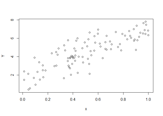
The data is illustrated in a scatter plot. When analysing the data using
lm() I get the following results
|
|
##
## Call:
## lm(formula = Y ~ x)
##
## Residuals:
##      Min       1Q   Median       3Q      Max
## -2.49576 -0.61718 -0.08426  0.60519  2.07532
##
## Coefficients:
##             Estimate Std. Error t value Pr(>|t|)
## (Intercept)   1.8667     0.2093   8.918 2.69e-14 ***
## x             5.1762     0.3560  14.540  < 2e-16 ***
## ---
## Signif. codes:  0 '***' 0.001 '**' 0.01 '*' 0.05 '.' 0.1 ' ' 1
##
## Residual standard error: 0.9751 on 98 degrees of freedom
## Multiple R-squared:  0.6833, Adjusted R-squared:   0.68
## F-statistic: 211.4 on 1 and 98 DF,  p-value: < 2.2e-16
which gives me an estimate of the intercept & slope.
The equation corresponding to the model above can be expressed as
$$ Y = \beta_{0}+ \beta_{1}x_{1}+\epsilon $$ the model fit to the data
via lm() estimated that $\beta_0$ = 1.8667 and $\beta_1$ = 5.1762.
While, the model equation is useful in some ways (e.g. easy to understand) it is also highly specific and only pertains to models that exactly like this one, which have an intercept and a slope. When conceptualising everything in the GLM-framework, we can do something much more powerful as we can generally write this model as
$$ Y = X\beta + \epsilon $$
which is the a valid description for all the different kinds of models & tests that fall under the GLM umbrella. Therefore we can use the same notation and tricks to deal with a wide variety of statistical problems. All that we have to do to analyse data following this notation is to create the design matrix $X$.
|
|
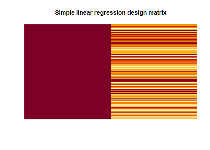
In the simple example above our design matrix has 1s for the intercept (i.e. $\beta_0$) and the values of our variable $x$ for the second column representing $\beta_1$.
When we have this, estimating the $\beta$s is very simple, assuming that $X^\intercal X$ is invertible (for an inverse of $X^\intercal X$ to exists $X$ must have full column rank, see Glossary for explanation or the YouTube video that I added), using this equation:
$$ \hat{\beta} = (X^\intercal X)^{-1} X^\intercal Y$$
Note that is what we get if we premultiply $Y = X\beta + \epsilon$ by $X^\intercal$:
$$ X^\intercal Y = X^\intercal X\beta$$ which is a neat trick that allows us to invert the matrix.
In R this would look like this:
|
|
Fortunately, using this equation we get the same values for $\beta_0$ = 1.8667 and $\beta_0$ = 5.1762.
Quick side note: solve() can only invert matrices that are square
(e.g. 3 x 3) directly
$$ A = \begin{bmatrix} 2 & 5 & 3 \ 4 & 0 & 8 \ 1 & 3 & 0 \end{bmatrix} $$
in this case
$$ A^{-1} = solve(A) = (A^\intercal A)^{-1} A^\intercal$$
|
|
So the trick of transposing and then multiplying the matrix with itself is something we have to use because our design matrix $X$ are typically not square.
Moving on, estimates for $Y$ can be calculated like this
$$ \hat{Y} = \hat{\beta_{0}} + \hat{\beta_{1}}x_{1}$$
or in matrix notation
$$ \hat{Y} = X\beta $$
In R this works simply by
|
|
The residuals can be obtained like this
$$ e = Y - \hat{Y} $$
|
|
To calculate the test statistics like $t$ we also need an estimation of the variance of the residuals
$$ \hat{\sigma}^2 = \frac{e^\intercal e}{N-p} $$ where $N$ is the number of rows and $p$ is the number of columns of the design matrix $X$.
|
|
In our case $\hat{\sigma}^2$ is 0.9508.
With the help of contrasts that are row-vectors with length $p$ we can test hypotheses as t-tests (or even as F-tests).
For instance, if we want to test if the intercept ($\beta_0$) is zero i.e. $H_o: \beta_0 = 0$, we can use the following contrast
$$ con_1 = \begin{bmatrix} 1 & 0\end{bmatrix}$$ If we want to test if our slope ($\beta_1$) is zero i.e. $H_o: \beta_1 = 0$, we use the following contrast:
$$ con_2 = \begin{bmatrix} 0 & 1\end{bmatrix}$$ Both hypotheses can be expressed more generally as $H_0: c\beta =0$. In R, we simply need to do
|
|
The $t$-statistic is then calculated by
$$ t = \frac{con\hat{\beta}}{\sqrt{con(X^\intercal X)^{-1}con^\intercal \hat{\sigma}^2} }$$
This looks more scary then it is. The numerator in case for $con_1$ is simply our $\beta_0$ estimate.
|
|
$c_1\hat{\beta}$ = 1.8667. The denominator is the standard error of the estimate. Which can be calculated by
|
|
so $\sqrt{con_1(X^\intercal X)^{-1}con_1^\intercal \hat{\sigma}^2}$ is 0.2093.
|
|
So like above when calculated with lm() $t$ = 8.9182.
Just to demonstrate, we also get the correct values for our second contrast:
|
|
$t$ = 14.54.
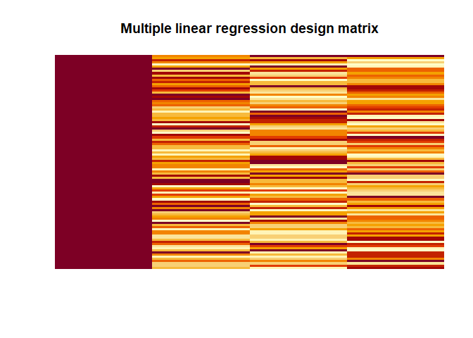
Multiple linear regression
Within the GLM-framework, we can also run multiple regression models and most importantly F-tests.
|
|
|
|
##
## Call:
## lm(formula = Y ~ x1 + x2 + x3)
##
## Residuals:
##     Min      1Q  Median      3Q     Max
## -2.2840 -0.6754 -0.0352  0.7310  2.2748
##
## Coefficients:
##             Estimate Std. Error t value Pr(>|t|)
## (Intercept)   2.2686     0.3515   6.454 4.43e-09 ***
## x1            4.6536     0.3740  12.442  < 2e-16 ***
## x2            0.2280     0.3633   0.628    0.532
## x3           -4.0781     0.3800 -10.732  < 2e-16 ***
## ---
## Signif. codes:  0 '***' 0.001 '**' 0.01 '*' 0.05 '.' 0.1 ' ' 1
##
## Residual standard error: 1.02 on 96 degrees of freedom
## Multiple R-squared:  0.741,  Adjusted R-squared:  0.7329
## F-statistic: 91.55 on 3 and 96 DF,  p-value: < 2.2e-16
|
|
|
|
Again we get the same values as with lm() 2.2686, 4.6536, 0.228,
-4.0781.
If we want to test $H_0: \beta_1 = \beta_2 = \beta_3 = 0$ or in other words if any of the $\beta$s that are not the intercept are different from zero, then we can use the following contrast:
$$ con = \begin{bmatrix} 0 & 1 & 0 & 0 \ 0 & 0 & 1 & 0 \ 0 & 0 & 0 & 1\end{bmatrix} $$
|
|
The test statistics is then calculated by
$$ F = (con\hat{\beta})^\intercal [rcon(\hat{Cov}(\hat{\beta}))con^\intercal]^{-1}(con\hat{\beta})$$
where $r$ is the rank of the contrast matrix/vector $con$,
|
|
which in our case is 3 as there are 3 independent columns in $con$ and
$$ \hat{Cov}(\hat{\beta}) = (X^\intercal X)^{-1}\hat{\sigma}^2 $$
Now we can calculate our F-value by hand:
|
|
In this case, $F$ = 91.5454, which can matches the one that lm() spits
out.
Special cases
The GLM is also powerful not only for the these regression models but also for a number of special cases that we often use for imaging.
One sample t-test
|
|
In this model $\beta_1 = mean(Y)$ = 4.4319552. As calculated when we use
t.test(), the $t$-value is 26.2878. $H_0: \beta_1 = 0$.
|
|
##
##  One Sample t-test
##
## data:  Y
## t = 26.288, df = 99, p-value < 2.2e-16
## alternative hypothesis: true mean is not equal to 0
## 95 percent confidence interval:
##  4.097429 4.766481
## sample estimates:
## mean of x
##  4.431955
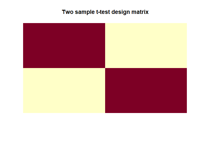
Two sample t-test
|
|
|
|
In this model $\beta_1 = mean(y_1)$ and $\beta_2 = mean(y_2)$ which are
-0.0807, 0.2204 (the group averages). As calculated with t.test(), the
$t$-value is -2.3043. $H_0: \beta_1 - \beta_2 = 0$.
|
|
##
##  Two Sample t-test
##
## data:  y1 and y2
## t = -2.3043, df = 198, p-value = 0.02224
## alternative hypothesis: true difference in means is not equal to 0
## 95 percent confidence interval:
##  -0.55875369 -0.04341614
## sample estimates:
##   mean of x   mean of y
## -0.08068517  0.22039974
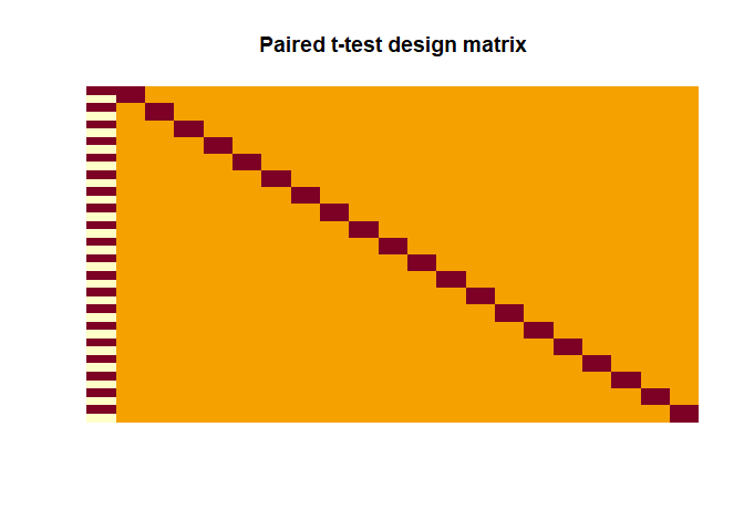
Paired t-test
|
|
|
|
Here the contrast has to be
$$ con = \begin{bmatrix} 1 & 0 & 0 & 0 & \cdots & 0\end{bmatrix}$$ in
order to test $H_0: \beta_{diff} = 0$. As calculated with t.test(),
the $t$-value is 0.2388.
|
|
##
##  Paired t-test
##
## data:  y1 and y2
## t = 0.2388, df = 19, p-value = 0.8138
## alternative hypothesis: true difference in means is not equal to 0
## 95 percent confidence interval:
##  -0.6600471  0.8300599
## sample estimates:
## mean of the differences
##              0.08500641
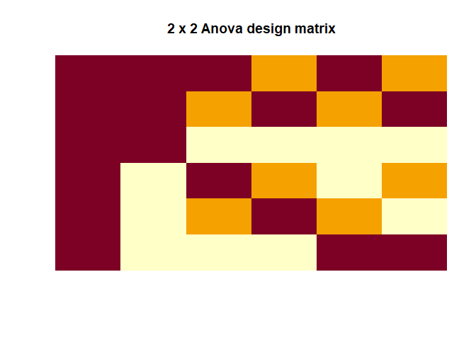
Two-way ANOVA
|
|
|
|
Again, we can compare this to what base R functions estimate:
|
|
##                    Df Sum Sq Mean Sq F value Pr(>F)
## A_factor            1  188.2  188.22  175.42 <2e-16 ***
## B_factor            2  161.5   80.77   75.27 <2e-16 ***
## A_factor:B_factor   2  220.7  110.37  102.86 <2e-16 ***
## Residuals         114  122.3    1.07
## ---
## Signif. codes:  0 '***' 0.001 '**' 0.01 '*' 0.05 '.' 0.1 ' ' 1
which fits with our $F$-values that we estimated 175.4229, 75.2738, 102.8615.
Does the contrast weighting matter for the test-statistics?
One thing I asked myself when thinking about it, is whether matters and if not why doesn’t it matter how we have weigh our contrast. Often we read that the contrast $con_1$ gives use the average of the two betas but is this true? Let’s look at this for two-sample $t$-test.
|
|
when we look at the numerator for $con_1$, which is supposed to represent the average of both $\beta$s we see that it is 0.164 but the average of $Y$ is only 0.082. So, in fact we get the average of the $\beta$s/groups times 2! We only actually get the true average when we use $con_2$ as a contrast, here the numerator is indeed 0.082. Does this actually matter for the test statistic? Well, no because as we scale the numerator by two, we also scale the denominator by the same amount and it cancels each other out. Both contrasts get exactly the same $t$-value of 0.565176.
Covariance matrix of the residuals
So, while reading through the Poldrack’s book I kind of stumbled over the concept of the covariance matrix of the residuals, which this is an important concept for time-series and heterogeneous variances but I didn’t really understand it when I am honest. So here I am trying to explore this:
The variance-covariance matrix is given by (in Kutner, 2005 this is written as $\sigma^2{\epsilon}$ and $MSE$ is used for estimation)
$$ \hat{Cov}(\hat{\epsilon}) = \sigma^2(I-H) $$
where $I$ is the identity matrix and $H$ is the so-called hat matrix that essentially can be used to transform $Y$ into $\hat{Y}$ directly (i.e. $\hat{Y} = HY$).
$$ H = X(X^\intercal X)^{-1}X^\intercal$$
Let’s calculate the covariance-variance matrix for our last example (the 2 x 2 ANOVA)
|
|
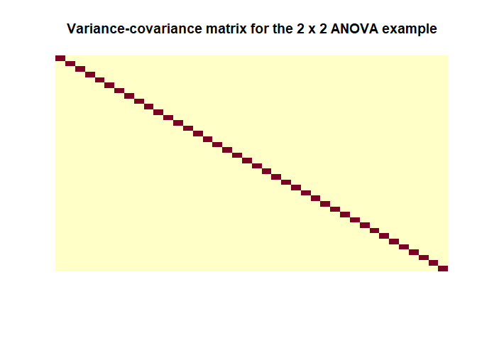
as when using the formula we can see $\hat{Cov}(\hat{\epsilon})$ is indeed a matrix with values close to zero off the diagonals and the a constant value on the diagonals. Important note: this estimation is only based on the design matrix $X$ so it doesn’t represent a feature of the data because we can’t really estimate the covariance of the true residuals so calculating this for your model will tell you nothing. It is simply an important assumption that is made about the data in order for everything to check out as intended. I found this helpful post about it.
A example design matrix for fMRI
The last thing directly related to the GLM that I wanted to explore is what first-level fMRI GLMs typically look like. That is because the actual design matrix used when fitting a GLM to fMRI data are the regressors (i.e. time points) convolved with the HRF. This is based on explanations and code from Jeanette Mumford (video & code). Here I illustrate constructing regressors for an first-level fMRI analysis. Note that in principle you want to convolve your events (onset + duration) with the HRF at a higher temporal resolution but for what ever reason this doesn’t seem to work well with the package that I am using. (Update: This is soon to be fixed by the developers.)
|
|
The results can be visualised as
|
|
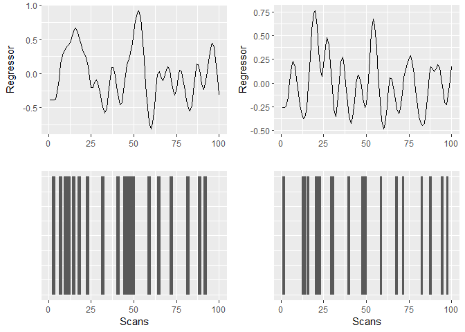
The resulting design matrix as used for fMRI would look like this
|
|
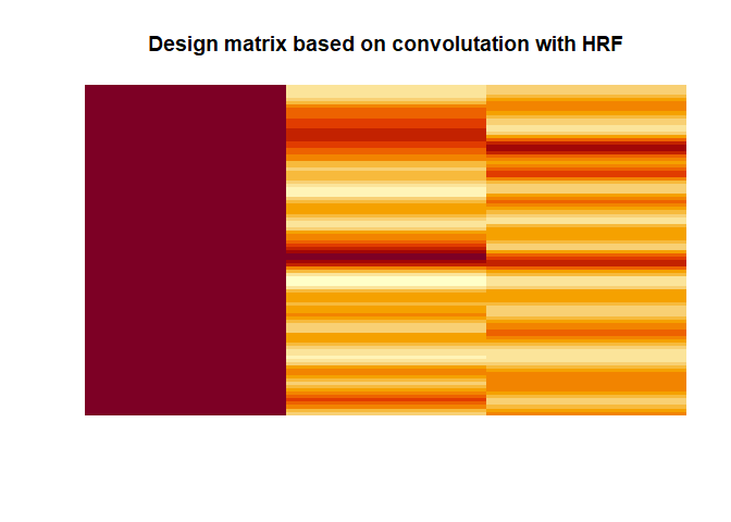
This, in other words a simple multiple regression model with continuous regressors, is what actually would be used to model the brain responses (at least for the first level analysis). Again, this ignores the problem of auto-correlation in the time-series and that the assumption about the covariance variance matrix of the residuals would not hold without extra steps, which are ignored here.
Multiple testing problem
The last problem I looked is not really GLM specific but important for fMRI analyses. When doing mass-univariate statistics on the brain, this usually means that we in fact run more than 100,000 individual tests as at least one test is run per voxel in the brain image. This is illustrated with this example of 2D fake brain image:
|
|
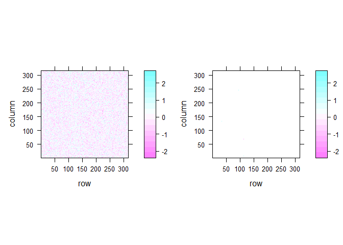
Even if there is no true effect, there are quite a number of significant voxels in that 2D brain image even when I smoothed it (13 voxel). In the unsmoothed image, we get a number of significant cases that is pretty much expected given the number of tests that we simulated (5060 voxels or 5.07 %). In real fMRI the false positive rate is obviously not that bad because voxels are not actually independent but it is still an important issue.
Note I am only discussing voxel-wise corrections but many of the concepts below also work for cluster level.
Calculate FWE
As defined below, FWE = chance of 1 more significant voxels in the brain and we want that to be 5%. So how much is the FWE in my completely fictional example for smoothed image.
|
|
Even with this relatively low number of significant voxels in each smoothed image the FWE is very high with 99.9 %.
FWE correction
As noted elsewhere Bonferroni is far too conservative. Two alternatives to correct for the FWE rates are random field theory (RFT) & permutation testing.
Random field theory
Famously, RFT is quite complex so I am not trying to dive much deeper into this matter other than repeating an equation taken out of Poldrack et al. (2011):
$$p_{FWE}^{vox} \approx R \times \frac{(4ln(2))^{3/2}}{(2\pi)^2}e^{-t^2/2}(t^2-1)$$
where $R = V/(FWHM_xFWHM_yFWHM_z)$ (RESolution ELement aka RESEL) and $V$ is the search volume.
Permutation tests
Permutation tests are something that can be relatively easily be simulated. This can be done by creating a number of brain images and saving the max-value test statistic in this image. I already did this while calculating the FWE above.
|
|
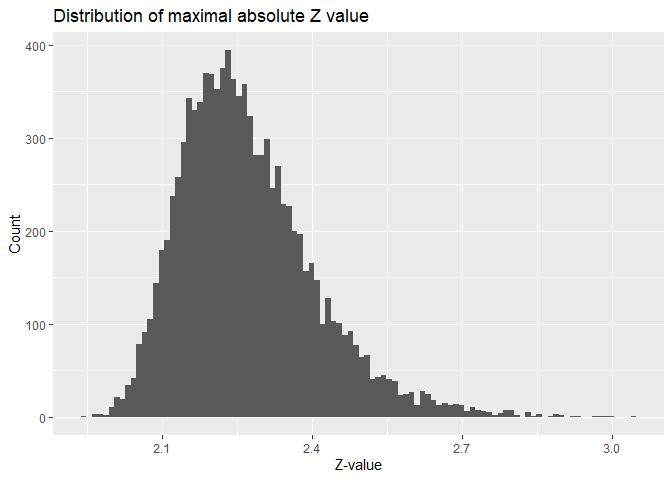
The FWE-corrected $p$-value is simply the percentage of values that are larger than our test statistic in that distribution. Take for example a z-value of 2.2025748. The $p$-values are as follows:
- Uncorrected: 0.0276247
- Bonferroni corrected: 1 (the $\alpha$-level would be 5.0072104^{-7}). In other words, we would only count absolute z-values of 5.0260363 or higher as significant.
- Permutation corrected: 0.3366. Here we would count values of at least 2.5175497 as significant.
FDR
Another way to correct the p-value is using FDR for instance using Benjamini’s & Hochberg’s proecdure. To simulate this, we again take our fake 2D brain image and convert the z-values into p-values.
|
|
As a reminder, we have 13 voxels that are deemed significant. In Step 1 we have to sort our p-values from smallest to largest and assign a rank.
|
|
for Step 2 we calculate the critical value for each p-value using
$$ crit = (i/m)\times Q $$
- $i$ = rank of p-value
- $m$ = total number of tests
- $Q$ = your chosen false discovery rate, which we set to 0.05.
|
|
Step 3 we try to find row where the value of the p-value is lower than the critical value.
|
|
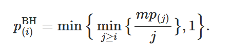
In this case, any(FDR_df$lower) is FALSE. Finally for adjusting a
p-value according to this procedure we can use
this
formula that I found:
|
|
This adjustment makes all our p-values 1. In more interesting example, we get this:
|
|
| p | rank | crit | lower | adjust_manual | adjust_adjust |
|---|---|---|---|---|---|
| 0.0010000 | 1 | 0.0045455 | TRUE | 0.0110000 | 0.0110000 |
| 0.0075637 | 2 | 0.0090909 | TRUE | 0.0416003 | 0.0416003 |
| 0.1600754 | 3 | 0.0136364 | FALSE | 0.3877979 | 0.3877979 |
| 0.1727596 | 4 | 0.0181818 | FALSE | 0.3877979 | 0.3877979 |
| 0.1762718 | 5 | 0.0227273 | FALSE | 0.3877979 | 0.3877979 |
| 0.2380772 | 6 | 0.0272727 | FALSE | 0.4364749 | 0.4364749 |
| 0.4092754 | 7 | 0.0318182 | FALSE | 0.5036225 | 0.5036225 |
| 0.4096089 | 8 | 0.0363636 | FALSE | 0.5036225 | 0.5036225 |
| 0.4120547 | 9 | 0.0409091 | FALSE | 0.5036225 | 0.5036225 |
| 0.6297573 | 10 | 0.0454545 | FALSE | 0.6927330 | 0.6927330 |
| 0.9008737 | 11 | 0.0500000 | FALSE | 0.9008737 | 0.9008737 |
Conclusion
Overall, I have to say that despite having dealt with these kind of questions & problems for years only really playing around with the equations in code helped me understand the concepts in deeper way. Hopefully, other people might also find this somewhat useful.
Glossary
- Rank = Number of independent columns in matrix or the number of dimensions in the output (if matrices are seen as transformations).
- Full rank = Rank is as high as the number of columns.
- FWE (rate) = “is the chance of one or more false positives anywhere in the image.” (Poldrack et al., 2011, p. 117)
- Bonferroni = A correction where simply $\frac{\alpha}{number\ of\ tests}$ assuming the the tests are independent. This is a method to correct FWE.
- FDR = Expected proportion of voxels deemed significant that are false positives.