Comparing different methods to calculate Bayes factors for a simple model
- Introduction
- Comparing the four BF methods
- Evidence for null hypothesis:
brmsvs.ttestBF() - How much more conservative is the
bmrsapproach? - Directed vs. non-directed hypothesis
- Conclusion
Introduction
In this post, I’d like to examine how different ways to calcualte Bayes
factors (BF) compare with each other for a simple model. This simulation
was run on my department’s HPC using the rslurm package: the
corresponding R code, data and .Rmd for this post are available.
For this simulation, I generated data of a within-subject model with two levels. The simulation comprised 10,000 iteration per effect size Cohen’s d (0.0, 0.5 and 0.8). Samples of 60 were generated with this function:
|
|
The equation of this model can also be written as:
$$y_{ji} = b_{0j} + x_{i}N(d, 1)$$
where $y_{ji}$ is the value for the j-th subject and the i-th level,
$b_{0j}$ a subject specific intercept and $x_{i}$ is the level
dummy-coded (0 & 1) that is multiplied with a value drawn from normal
distribution with a mean of $d$ (0.0, 0.5 or 0.8) and a standard
deviation (SD) of 1. For the brms model, we scaled the data to a mean
of 0 and an SD of 1.
I then compared 4 ways to calculate a BF to examine the mean difference of the two levels.
ttestBF(): For the first method, I usedttestBF()from theBayesFactorpackage. This is a widely used Bayesian implementation for the classical t-tests (Rouder et al., 2009). For this simulation, I used the standard medium rscale ofsqrt(2)/2≈ 0.707. Note that this approach uses different priors (Cauchy/Jeffry’s prior) and likelihood functions than thebrmsmodels below. So, I expect differences but it still can be used as a reference point.
The reaming four methods are all based on the same brms
model.
|
|
For the intercept and the beta value, I placed a normal prior, N(0, 1):
|
|
To make full use of our HPC, I only used 1 chain per model. Each run used 36000 samples in total of which 3000 were for warm-up.
bayes_factor(): For this method, I compared the full model with a null model that did not include x.
The other two methods are based on an approximation of the BF that does not calculate the marginal likelihood but instead the point density at zero for the prior and the posterior distribution, which is known as the Savage-Dickey ratio.
-
hypothesis(): This function is a Savage-Dickey ratio implementation from thebrmspackage. Can be used like thishypothesis(model_full, 'x = 0'). -
manual: This approach estimates the point density via Logspline Density Estimation. This is adapted from code from Wagenmakers et al. (2010) and can be found on his website. This method used
logspline()from thepolsplinepackage. Note that instead of also estimating the point density from the prior samples as generated bybrms, I just used the respective base functiondnorm().
|
|
This method by the way also allows to easily calculate the BF for directed hypotheses (i.e. d = 0 vs. d > 0):
|
|
See Wagenmakers et al. (2010) for more information on this. This will also examined at the end of this post.
Comparing the four BF methods
Below you find the scatterplots comparing the different ways of estimating a BF. To aid illustration, the data is presented in natural log-space. Each plot contains up to 10,000 data points.
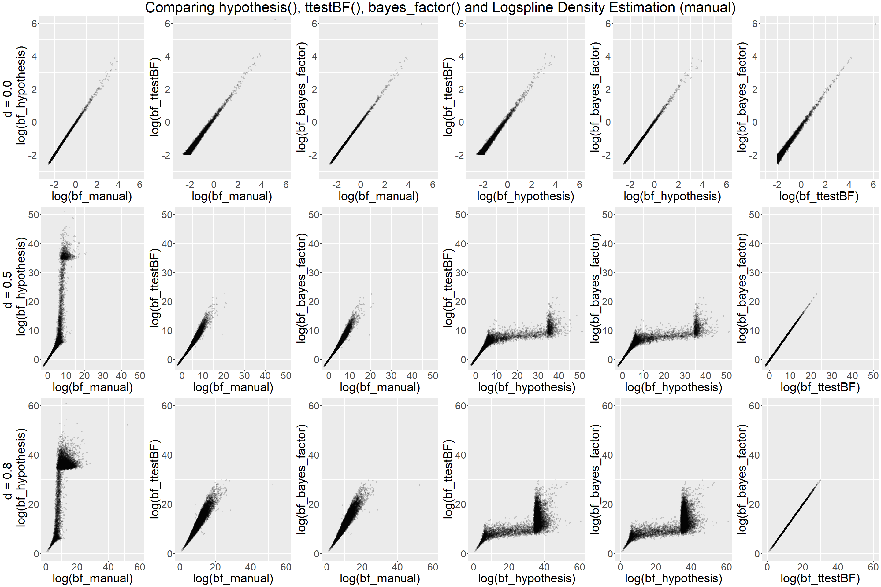
The the scatterplots reveal when d = 0.0 that all methods compare well
with each other. In contrast for d = 0.5 and d = 0.8, hypothesis()
function starts to break down at around BF10 = exp(5) ≈ 150 and only
returns extremely inflated estimates. The manual method via Logspline
Density Estimation leads to more stable estimates, while the spread
(e.g. manual vs. bayes_factor()) also becomes larger at around BF10 =
exp(7) ≈ 1100. However, the estimations are not skewed as the ones
returned by hypothesis(). In that sense, the manual method based on
Logspline Density Estimation is superior. The reason for that is that
hypothesis() does not perform well if the estimation is only based on
very few values around zero, which happens when the distribution is
shifted away from zero.
As already noted above, there ttestBF() and the brms model have
different priors and likelihood functions, but comparison with the BF
from ttestBF is still useful to examine if they point in the same
general direction and indeed they do. In fact, the correlation for d =
0.5 and d = 0.8 is extremely linear. However, we also see that in the
top right corner that for d = 0.0 there is an interesting increasing
spread towards low values (e.g. see ttestBF() and bayes_factor()).
The reason for this spread reflect the different performance of the
methods to produce evidence for H0 (see next section).
All in all, the manual method does a good job with the advantage that it
is a lot after than bayes_factor() providing sensible estimates in
cases that matter most to use as psychologists/cognitive neurosciences.
In most circumstances, it doesn’t really matter if a BF10 is 1500 or
only 1100.
Evidence for null hypothesis: brms vs. ttestBF()
To illustrate the difference between brms and ttestBF(), I binned
the BF into 8 categories and compared their
frequencies.
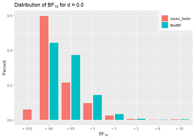
A look at the two distributions shows that the brms model with unit
prior of N(0,1) leads to stronger evidence for the null when the null
hypothesis is true than ttestBF() with its Cauchy/Jeffrey’s prior
implementation does. Zero percent of ttestBF()’s BF10 were < 1/10.
This highlights the more conservative nature of the brms model. As a
comparison, we can look at the distribution of BF10 when effect size is
d =
0.5.
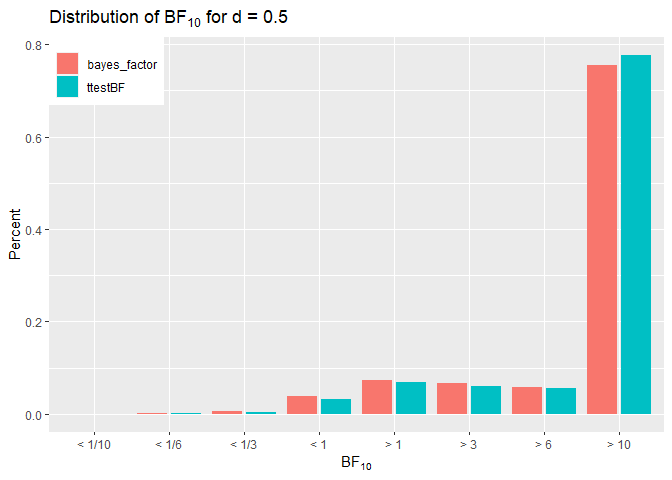
In this case the percentages are very similar despite being more
conservative, the bmrs model often leads to the same conclusion. Note
that for d = 0.8 all BF10 were above 10, hence they are not displayed
here but this illustrated that brms is doing well in these cases as
well.
How much more conservative is the bmrs approach?
The conservative nature can be illustrated by examining the distribution
of the ratios between both BFs
(ttestBF()/bayes_factor()).
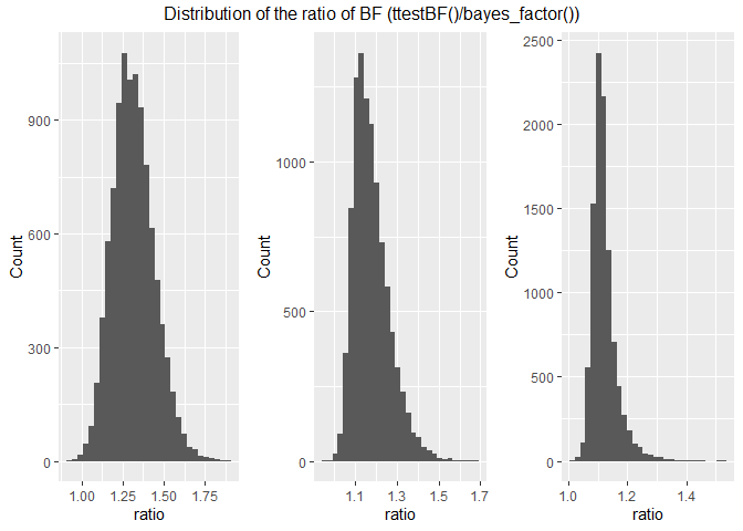
The distributions of ratios show that the brms model more conservative
than ttestBF() but as the effect size increase the max ratio drops
from 1.8 to 1.4. Median values are 1.308, 1.162 and 1.113 for a d of
0.0, 0.5 and 0.8, respectively. It can be seen that the unit-prior in
brms models regularises much more for lower d-values than ttestBF(),
which is a good thing if the aim is to provide evidence in favour of the
null hypothesis.
Directed vs. non-directed hypothesis
On each run in these simulations, I also estimated the order-restricted BF (i.e. BF for directed hypothesis) that d = 0 vs d > 0.
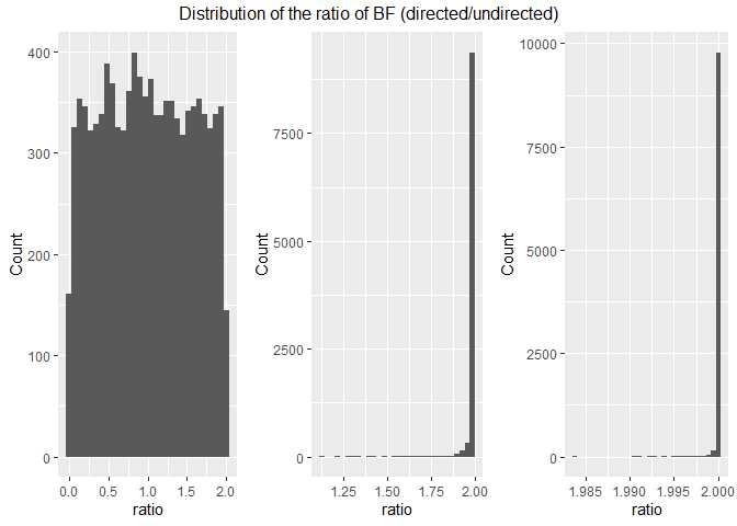
This shows that when the null is true, the order-restricted BF is much lower (median of 0.989) compared to d = 0.8 because follows are uniform distribution. For positive effect sizes (d = 0.5 & d = 0.8), the ratio is very close to 2.
Conclusion
All in all, that simulation showed that the brms model with unit-prior
are more conservative than ttestBF() but lead to similar conclusions
if d > 0. With respect to the four models, I would that the manual
implementation is usually enough as it and easy, quick and intuitive way
to calculate a BF. It definitely out performs the hypothesis()
function that easily breaks down if the posterior distribution has
little overlap with zero. Furthermore, hypothesis() does not work well
for priors that are hard to sample e.g. Cauchy prior. This is an issue
that has been previously
discussed
but my tests show that the manual method gives quite reasonable
estimates in this scenario.