The priors that I use for logistic regression now
Problem
In my power simulation of the U-shape experiment, I noticed that the suggested priors (click here) actually do not work very well for Bayes Factor (BF) analysis as they are too flat and hence BF are too conservative. That is because uniform or very flat priors lead to less evidence in favour of the alternative hypothesis. Even though undoubtedly Bayesian models and Bayesian evidence does not have to tell us the exactly the same things that frequentist statistics do, however I do think it important to have some level of congruency as well as being clear what kind of sample sizes and effects we actually need to reach certain criteria that are standard in my field as valid evidence (p < 0.05, p < 005, $BF_{10}$ > 6 or $BF_{10}$ > 10). In this document, I therefore report my investigation how some characteristics of priors relate to evidence that they are associated with.
Disclaimer, this post is not mentioned as an exhaustive paper but merely my own attempt to come up with sensible priors for the kind of models that I run. Especially since there doesn’t seem to be much out there on this question. With that being said maybe it will be useful for other people and I am more than happy to get feedback/corrections/questions or even be told that my reasoning is completely flawed.
A word on logistic regression
Before we can talk about priors we need to talk about logistic regression and what the regression coefficients and their size mean. A great explanation of what probabilities, odds and log odds mean in the context of logistic regression can be found here.
$$logit(p) = log(\frac{p}{1-p}) = \beta_0 + \beta_1 x_1 + \cdots + \beta_k x_k.$$
The equation above describes a logistic regression model with several predictors. The $\beta$-values have been logit transformed and represent log-odds. Odds are ratios of probability. So if you have a 75 % success rate in something that translates to odds of .75/(1 - .75) = 3 or log-odds of log(3) = 1.098612.
As in normal regression, the regression coefficient is relative to the scale of the predictor variable (e.g. height in cm). For instance, a coefficient of 1.098612 would mean a 200 % increase in odds to have success per cm increase in hypothetical example.
Gelman (2008) suggest to scale the predictor variables to have a mean of 0 and a SD of 0.5. In another hypothetical example, we scale our data accordingly and get a regression coefficient of 0.2231436 or in odds 1.25. This would mean for every time our predictor variables increases 2 SDs the odds increase 25 %.
These circumstances illustrate that it is sensible to set some boundaries on our priors, which essentially means that we don’t expect coefficients beyond a certain range in the type of work we do. This is a thought I will revisit in the conclusions to justify the prior I will choose.
Influnece of degrees of freedom for Student’s distrubution.
In his recommendation for priors Gelman now follows Ghosh et al. (2015) and recommends a student distribution with degrees of freedom (df) between 3 and 7 with a scale of 2.5. For illustration of how Student’s distribution changes with df, I created this graphic.
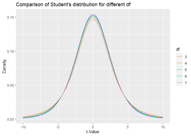
The figure above illustrates that there is an inverse relationship of the density at the peak and the density at the tails. For comparing df = 3 with df = 7, at the mode of the distribution the df = 7 is higher, while at the tails the distribution with df = 3 is higher. Increasing the df basically essentially gives more weight to extreme values. In the following, I examine how choosing different df affects evidence in a BF analysis.
Background on pre-simulation
The data in the simulations were generated data with this function:
# Function used to generate data
data_generator <- function(numSub, beta0, beta1){
  # Create DF and also scale x
  df <- data.frame(sub  = rep(1:numSub),
                   x    = rnorm(numSub))

  # Scaling based on https://github.com/stan-dev/stan/wiki/Prior-Choice-Recommendations
  # Mean = 0 and SD = 0.5
  df$s_x <- (df$x - mean(df$x))/(sd(df$x)/0.5)

  # Predicting memory
  z     <- beta0 + beta1*df$s_x # Regression in log odds
  pr    <- 1/(1+exp(-z)) # Convert to probability.
  df$y  <- rbinom(numSub, 1, pr)
  return(df)
}
Note that I follow Gelman’s (2008) recommendation about scaling the variable to have standard deviation (SD) of 0.5. The considerations concerning the priors therefore only pertain to this scaling. For the first simulation, I used the recommended 2.5 for the scale of the Student’s distribution (1000 iterations per condition).
priors_student_1  <- c(prior(student_t(3, 0, 10) , class = "Intercept"),
                       prior(student_t(3, 0, 2.5) , class = "b"))
In a second simulation, I contrasted the results with a scale of 1 for the Student’s distribution (5000 iterations per condition).
priors_student_1  <- c(prior(student_t(3, 0, 10) , class = "Intercept"),
                       prior(student_t(3, 0, 1) , class = "b"))
In both simulations I used the following df of 3, 4, 5, 6 and 7. The simulations included simulated sample size of 100 for all simulations. The BRMS model that was used for fitting was this one:
brm(y ~ s_x,
    data = df,
    prior = priors_student_1,
    family = bernoulli(),
    chains = 1,
    save_all_pars = TRUE,
    sample_prior = TRUE,
    save_dso = TRUE,
    seed = 6353)
Analyse simulation
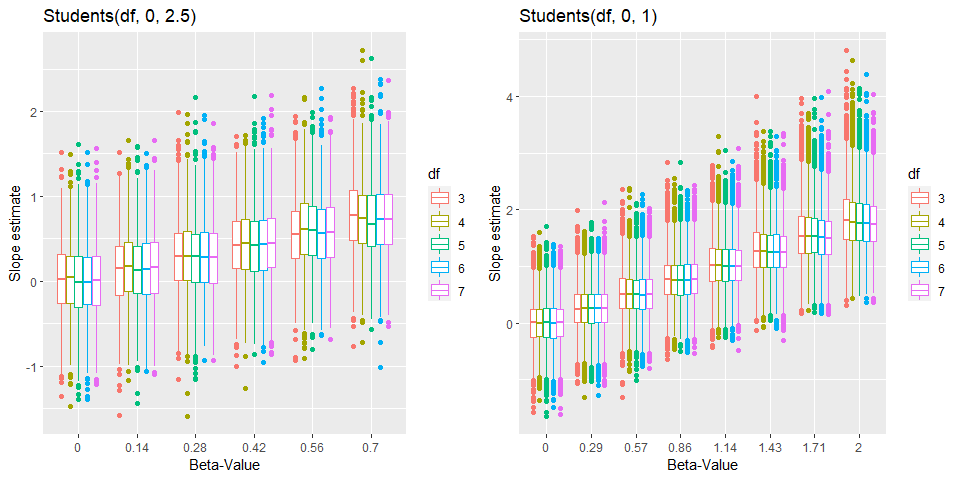
Simulation 1 (Scale = 2.5)
In this first simulation, I used $\beta_1$ between 0 and 0.7. The average FPR for a $BF_{10}$ > 6 for the priors with this scale is 0.0078 (0.001924) showing in general that this method is more conservative than a frequentist model would be. One obvious reason for this that the BF in contrast to the p-value is not uniformly distributed and it gets smaller and smaller with more data (for a null effect). In my frequentist simulation (see below), the nominal FPR was 0.045 for p < 0.05.
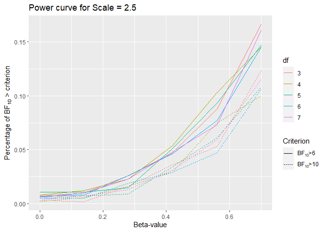
This power curve shows how badly the prior performance is. Even with a beta of 0.7 or odds of exp(0.7) = 2.013753, we only barely get past 15%. This is quite different from what we would get if we used frequentist models. That the prior is too wide contributes to the general conservatism problem of BF analysis, as I show in the next simulation.
Simulation 2 (Scale = 1)
In the next step, I ran a simulation with scale parameter of 1. To illustrate the difference between a scale of 2.5 and a scale of 1. Here both plotted on the same axis. For comparison, I also overlaid a normal prior, N(0, 1) illustrated by the dashed line.
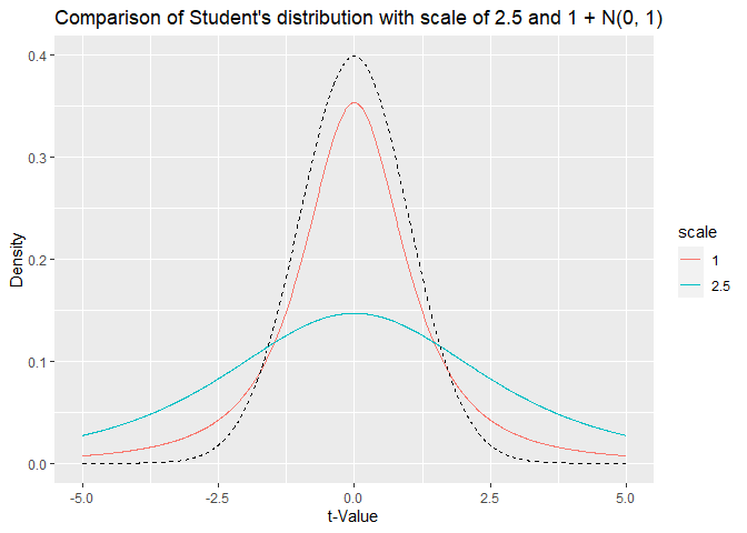
The student’s distribution with scale of 2.5 is far too wide explaining the low ‘power’ for $BF_{10}$ > 6. To see, how a prior with scale of 1 behave I ran Simulation 2. In this simulation, the $\beta_1$-values range from 0 to 2.
The average FPR for a $BF_{10}$ > 6 for the priors with this scale is 0.01288 (0.00111), which is still quite low compared to frequentist models.
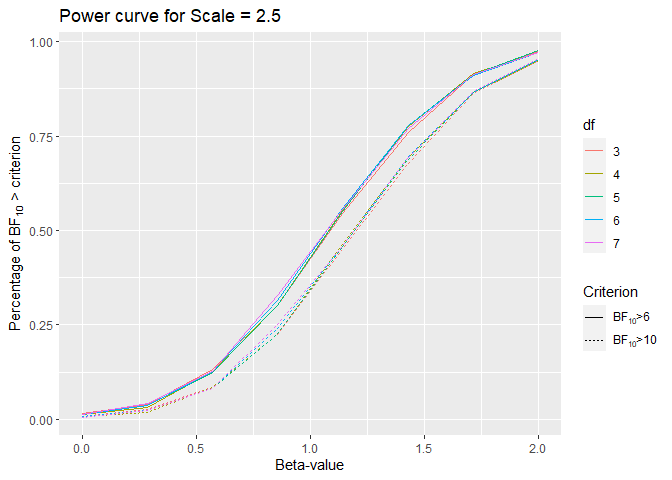
Looking at the power curve it seems that there is no big difference for different df.
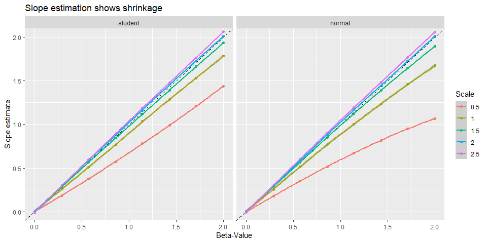
Comparison of slope estimation
In addition, we can look at the shrinkage properties. By comparing the true and the average estimated slope in scatter plot.
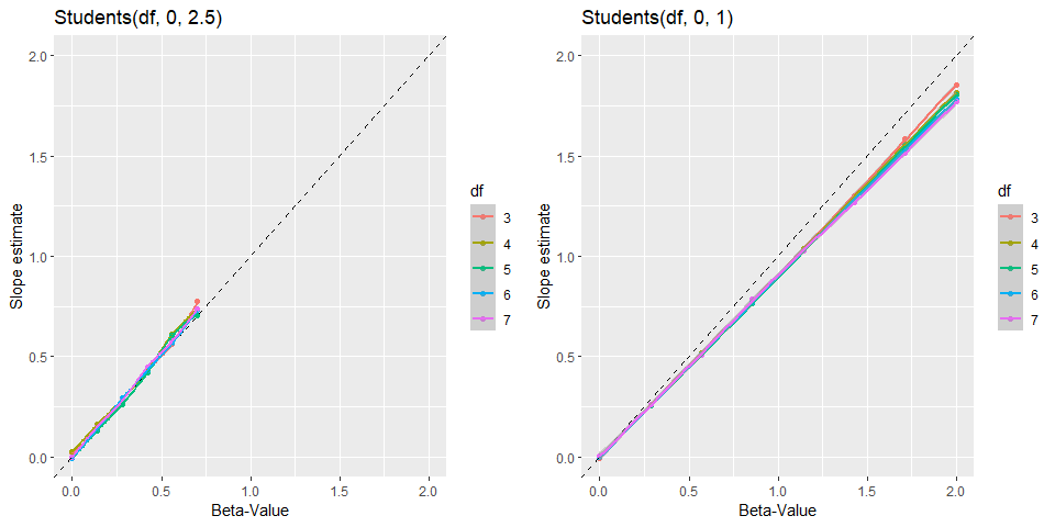
Despite the different ranges (0 to 0.7 and 0 to 2) in the simulations, it is obvious that narrower priors leads to more shrinkage toward zero. This is probably a good feature as this protects us from overestimating the effect.
Interim conclusion
My interim conclusion is that the suggested scale of 2.5 is too wide for BF analysis. Hence, I will run another simulation comparing normal versus student priors with scales of 1, 1.5, 2 and 2.5 to investigate this issue further.
Illustrative example
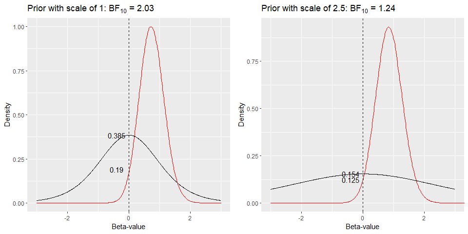
Before looking at the results, here is a quick illustration why this is the case. Above, two figures showing the analysis of the same data can be seen. The left one uses a scale of 1, the other one uses a scale of 2.5. The $BF_{10}$ are 2.03 and 1.24. The figures illustrate the Savage-Dickey method of calculating BF that is taking the ratio of the prior probability at zero and posterior probability at zero. While the posterior probabilities are similar with 0.19 and 0.125, the prior probabilities at zeros are very different 0.385 versus 0.154. This explains the difference in the BF that we get using both scales.
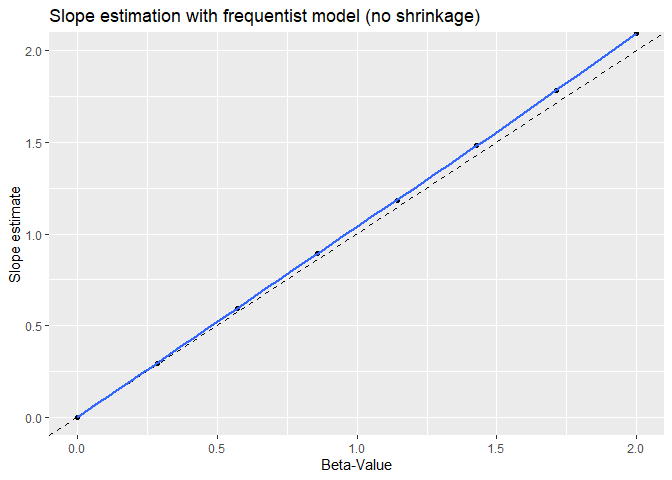
Frequentist comparison
In order to get a better idea how conservative the power curve from the Bayesian models are I also quickly run the same simulation with a frequentist model (10,000 iteration per $\beta_1$ value).
The model that I used was:
glm(y ~ s_x, data = df, family = "binomial")
Full simulation
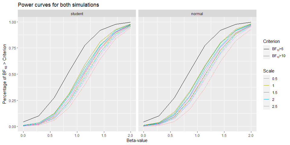
Above the power curves of this simulation can be found. The black line represents the power curve for equivalent frequentist model and shows that all priors are more conservative.
In contrast to Bayesian models, for the frequentist simulation we don’t find shrinkage of the estimator towards zero.
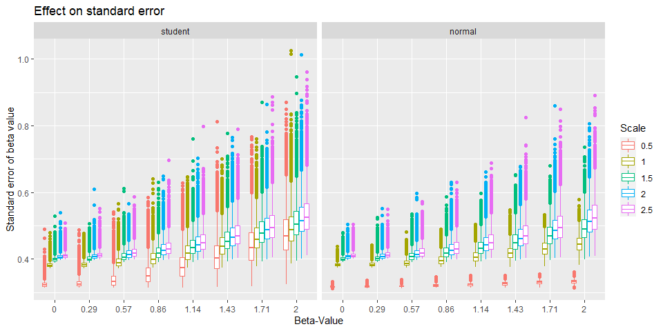
One thin that stand out when comparing the standard error is abnormally low for a prior with scale of 0.5 irrespective of the family.
One other number we can look at is the effective sample size. This number is not referring to the effect size of the coefficient but how many samples for analysis are effectively available. The more the better because estimation especially of the BF get more stable the more samples we’ve got.
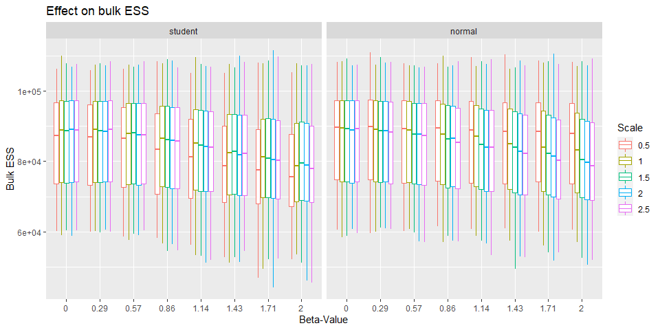
Here we see something interesting that is while the bulk ESS decreases for a scale of 0.5 as the beta-value get larger for the student prior, the opposite is true for the normal prior.
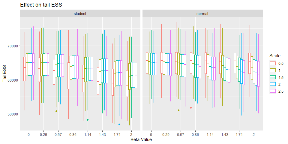
Yet again the reverse is true for tail ESS. This probably indicates that a scale of 0.5 is too narrow.
Conclusions
Several things can be learned from the simulations.
Now, if look which values these distributions include as likely by comparing the middle 95% of them, we see what that means in terms of odds and change per 2 SD increase in our predictor variable. Here are two tables for the upper boundaries (i.e. 97.5 %) for both normal and student distributions showing the regression coefficients as log odds.
Normal distribution:
| scale | coef | odds | change |
|---|---|---|---|
| 0.5 | 0.979982 | 2.66 | 166 |
| 1.0 | 1.959964 | 7.10 | 610 |
| 1.5 | 2.939946 | 18.91 | 1791 |
| 2.0 | 3.919928 | 50.40 | 4940 |
| 2.5 | 4.899910 | 134.28 | 13328 |
| scale | coef | odds | change |
|---|---|---|---|
| 0.5 | 1.182312 | 3.26 | 226 |
| 1.0 | 2.364624 | 10.64 | 964 |
| 1.5 | 3.546936 | 34.71 | 3371 |
| 2.0 | 4.729248 | 113.21 | 11221 |
| 2.5 | 5.911561 | 369.28 | 36828 |
One thing immediately apparent is that a scale of 2.5 still ‘treats’ values that correspond to a change of 13328 % & 36828 % per 2 SD on the predictor as likely. Generally, the fact that the student distribution has higher tails still allows for larger values. That is despite the fact that power for a normal prior versus a student prior (df = 7) with a scale of 1 are not systematically different. This is therefore an argument for using a student prior.
Furthermore, a student prior typically fits posterior distributions better (according to my limited experience), which is an advantage when trying to use previous posteriors as priors for new analyses. Using student priors throughout therefore eases comparison.
Even if for particular posterior distribution a normal is better fit then a student, then this will be alleviated by the fact the estimated df will just be very large as a student distribution will be identical for infinitely large df. To sum up, I will now use a student distribution with mean = 0, scale = 1 and df = 7 as the standard prior for logistic regression models.