The outset of the problem

In one of my project, I’d like to show that there is a U-shape relationship between two variables. The traditional way to do this would be to fit a quadratic model and test whether the quadratic term is different from zero. However, Simonsohn (2018) among other correctly points out that evidence for a quadratic fit is not enough and there might be situations where the quadratic term is not zero but there is no true u-shape.

To avoid this, Simonsohn proposed to use interrupt regression that tests whether each slope is different from zero. While the exact proposal (Robin Hood algorithm) might work well for frequentist statistics, it is not clear how we can adopt this for our Bayesian models. The main question being that it is unclear how to choose the correct breaking point. This is what I explore here extensively as a preparation for a pre-registration (for context click on link).

Explanation of the simulation

We identified two options to analyse our data with interrupted regression or more specifically how to find the best breaking point.

Option 1 is to split the data in half using a spline (or similar) to find the minimum/maximum in one half of the data and then analyse the other half of the data to test whether both slopes at a that point are significantly different from 0.

Option 2 is to use all data and test a whole range of points within an interval and then apply an appropriate correction for multiple testing. The aim of this document is to explore all the options and their implications. Also whether correction is necessary at all.

For option 1, I subset the simulated data to only include the middle 80% and then find the minimum via smoothing model. The smoothing model is the same used by Simonsohn’s two line test, which is a general additive model using a cubic regression spline. When I played around with it, it usually did a good job finding the point that would also be chosen via visual examination for the plotted loess line. I used only 80 % of the middle because especially when the $\beta_2$ is zero, the minimum was often the extreme points, which make a meaningful estimation impossible. An alternative for this could be to fit the smoothing model to the full range of the values but to only consider minima within the middle 80 % but this wasn’t tested here.

For option 2, I also restricted the range to same middle 80%, for which 10 breaking points evenly spaced out were examined. For each different $\beta_2$ I run 100,000 simulations.

Also note that some models couldn’t be estimated that is because some model didn’t return a minimum or only return NA. This happens particularly often in the frequentist models.

I start with frequentist mixed linear models to get an idea how both options compare in terms of how they behave and use those results as a perspective for the Bayesian implementation.

Like in the two-line test we fitted two individual models to the data. One model to get the p-value/BF for slope 1 that includes the breaking point. Since in this model slope 2 can’t contain the breaking point, we fitted another model where the breaking point is included in slope 2 but not slope 1, so that both slopes include the minimum/maximum and make best use of the data.

Note that links to the repository will be added at a later time point. If you read this in the far future and I haven’t done this yet, feel free to kick me.

Frequentist models

Using previous data to generated null data by shuffling

In order to find a way for appropriate multiple testing correction that is less severe than Bonferroni, I shuffled the 0 and 1 of original data (for context click on link) within subjects. This means that the average performance within subjects as in our actual data that we want to analyse after pre-registration is the same but the information for objects is lost. Due to the fact that in our example each subject only saw each type of object once, we cannot shuffle within both subjects and objects. After shuffling mixed linear models with a random intercept are fitted to the data following this equation

y ~ xlow + xhigh + high + (1 | sub).

Now, we examine the results of this simulation.

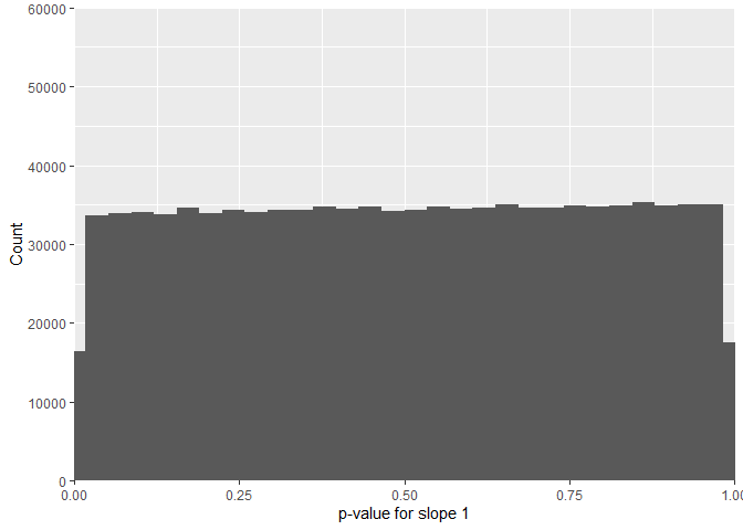
The FDR for U-shapes for null data generated by shuffling 0 and 1 within subjects is 3.796 % for mixed linear model with random intercept for subjects and objects. For slope 1 its 27.508 % and for slope 2 50.297 %. This shows an extreme asymmetry that can be traced down to the distribution of the p-values of the shuffled original data.

While the p-value for slope 1 is nicely uniform,

the p-values for slope 2 show extreme pikes at 0 and 1.

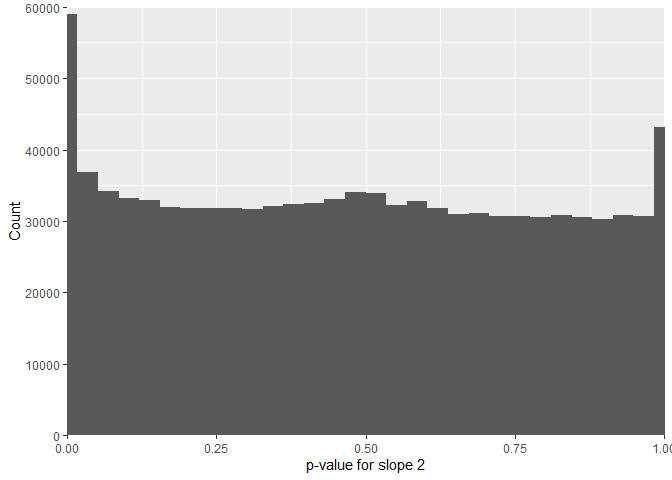
This is not due to an error in the code but due to the fact that the x-values are always the same with this shuffling method. When I randomly generated x-values like in the quadratic simulation below, we get the similar FPR for both slopes. To be sure about this, I ran a normal glm (without random effects) and got similar results, which means that the problem is not the model but the shuffled data where the x-values remain unchanged.

On a side note, I found for 18.7 % of the cases I had some kind of convergence warning while fitting the mixed linear model but since the glm showed the same results, this is not an important issue but shows how Bayesian models might be more robust against these kind of things.

One Slope < 0.05

With this simulation, I can now look for an alpha level for individual slopes so that we only have one or more significant slopes per iteration across the breaking points in 5 % of the cases.

For the shuffled data we get an alpha level of 0.0068 for individual slopes. This mean that we can accept the significance of individuals slopes if the p-value is below that level and still only be wrong in 5% of the cases. This is already slightly less conservative than a Bonferroni correction.

Quadratic simulation

To show that a) the data generated de-novo is not skewed like the shuffled above and b) to draw a power curve I ran another simulation that generated data via quadratic logistic regression with 100,000 iterations per $\beta_2$ (0, 0.175, 0.35, 0.525, 0.7). All simulations are run with sample size of 80. In the first step, I optimise the alpha level for the generated data in the same way I did above. The data was generated with this function:

The optimised alpha level for individual slopes is very similar for both slopes. Averaged it is p < 0.0081604.

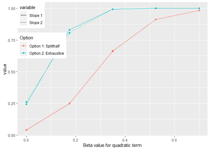
There are two things we can look at. First is how two both methods fair in detecting significant individual slopes in terms of power and FPR. The second thing we can look is how do the methods fair when the aim is to detect a U-shape (i.e. two significant slopes) especially once we corrected for multiple comparison.

Power curves for individual slopes

The FPR for generated data analysed with option 2 are 0.25073 and 0.26067.

In the following are the corrected slopes:

At this point we can also look at the distribution of p-values for those simulated x-values.

Also, just as a quick side note. When the data is generated instead of shuffled the p-values for both slopes follow a nice uniform distribution.

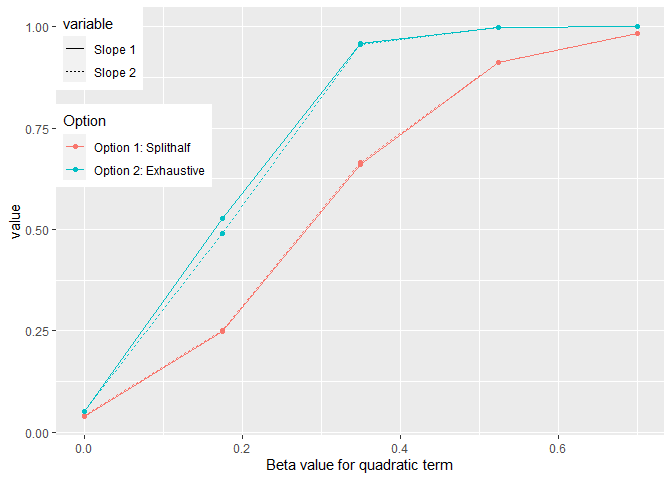
Power for detecting u-shape after correction

Now, we can examine how this correction procedure affects the abilitiy to detect a U-shape using both methods implemeneted as frequentist models.

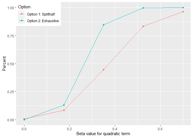
As can be seen above, option 2 fares much better than option 1 even after quite rigorous correction of multiple comparison.

One possible reason that option 1 fares poorly is that the estimation of the breaking point is very noisy. In fact the mean absolute difference is 0.7478701, which is quite large considering the range of values on the predictor variable in the simulation (min = -2.439 and max = 1.58). Typically, the values range between (+/- 1.2) though.

Conclusion

This simulation has shown that the FPR rate is indeed increased for individual slopes when testing 10 breaking points per analysis. However, this can be alleviated with appropriate correction of the alpha level for the individual slopes. Not that the correction is markedly less strict than a Bonferroni correction ($\alpha$) divided by the number of tests).

We can conclude that option 2 is preferable to option 1. Now in the next step, we apply the same approach to our Bayesian model and see how this behaves under the same circumstances.

Bayes factors

I used the same data generating function for this simulation and we also used 100,000 iterations with a $\beta_2$ of 0. For the Bayesian model I used these priors (for justification to use these priors see here)

priors  <- c(prior(student_t(7, 0, 10) , class = "Intercept"),
             prior(student_t(7, 0, 1) , class = "b")) 

and the following model.

# Preparation for interrupted regression (for more info see Simonsohn, 2018) of slope 1.
breakingPoints <- 0 # In this case I'd split it at zero. 
x              <- df$s_x 
df$xlow        <- ifelse(x <= breakingPoints, x - breakingPoints, 0)
df$xhigh       <- ifelse(x > breakingPoints, x - breakingPoints, 0)     
df$high        <- ifelse(x > breakingPoints, 1, 0)

# The model 
brm(y ~ xlow + xhigh + high,
    data = df,
    prior = priors,
    family = bernoulli()) 

Note that I didn’t add a random intercept because even when only using a total number of samples of 9000, adding a random intercepts would have increased the run time of this simulation significantly. The data was generated and scaled with this function:

This null data allows us to examine which $BF_{10}$ we could accept as individual slopes despite multiple testing and still retain a FPR of 5 % in total.

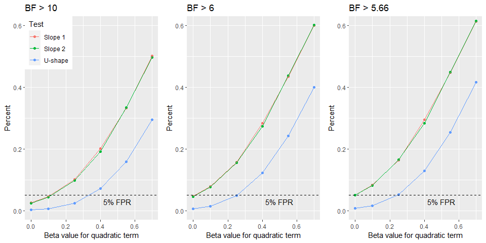
The results show in contrast to frequentist models where we have to lower the alpha level compared to the convention (p < 0.05) that we could accept $BF_{10}$ as low as 5.66 have the same FPR rate as we have for the frequentist models. Typically, journals accept a $BF_{10} > 6$ and sometimes a $BF_{10} > 10$ as sufficient evidence. The main reason for this stark discrepancy between frequentist and Bayesian statistics is that the latter are far more conservative than the former.

In our case, the FPR for individual slopes is 4.66 % with $BF_{10} > 6$ without any form of correcting for the fact that we ran multiple tests on the same data. This is based on 100,000 simulations.

Now we can examine the ‘power’ curve for our Bayesian model as function of using different $BF_{10}$ criteria.

Conclusion

The frequentist simulation showed without doubt that option 2 is better way of analysing the data. However, it also showed that testing multiple breaking points inflates the Type 1 error. The Bayesian simulation on the other hand provide us with evidence that is not an issue for this type of analysis as the FPR is much lower than that what we accept for frequentist models. That means that we could even lower the $BF_{10}$ to for accepting non-zero slopes below the commonly accepted evidence criterion of $BF_{10} > 6$ and still have a FPR of 5 % (i.e. $BF_{10} >$ 5.66). However, I do not propose to do this but stick with accepting individual slopes if they have a $BF_{10} > 6$, which provides me with enough confidence. Especially since we need both lines to surpass this level of evidence at the same time to conclude that we have U-shape.

In sum, I conclude that it is fine to take a $BF_{10} > 6$ as evidence for a non-zero slope even if I test 10 different breaking points for our data.