Bayesian sequential designs are superior
This post is based on a short talk that I gave at the MRC CBU on the 29 July 2020 for a session on statistical power. The slides of presentation can be found in my GitHub repository. This repository also includes the data and the scripts that were used to run the simulations and to create the figures. Most of this talk as well as of this post is based on Schoenbrodt & Wagenmakers’ (2018) fantastic paper that I encourage you to read as well as the other good articles in that special issue on Bayesian statistics.
So let’s see what number we need for having a high probability of getting strong evidence for a medium effect (d = 0.5) and a null effect (d = 0.0). This cane be done in the same way a traditional power analysis using frequentist statistics is run. That is we can calculate for which fixed sample size we get a Bayes factor (BF) surpassing a certain criterion in let’s say 80 % of the cases if repeated the data collection multiple times.
This procedure is illustrated in the figure below, which basically the same as a standard power calculation:
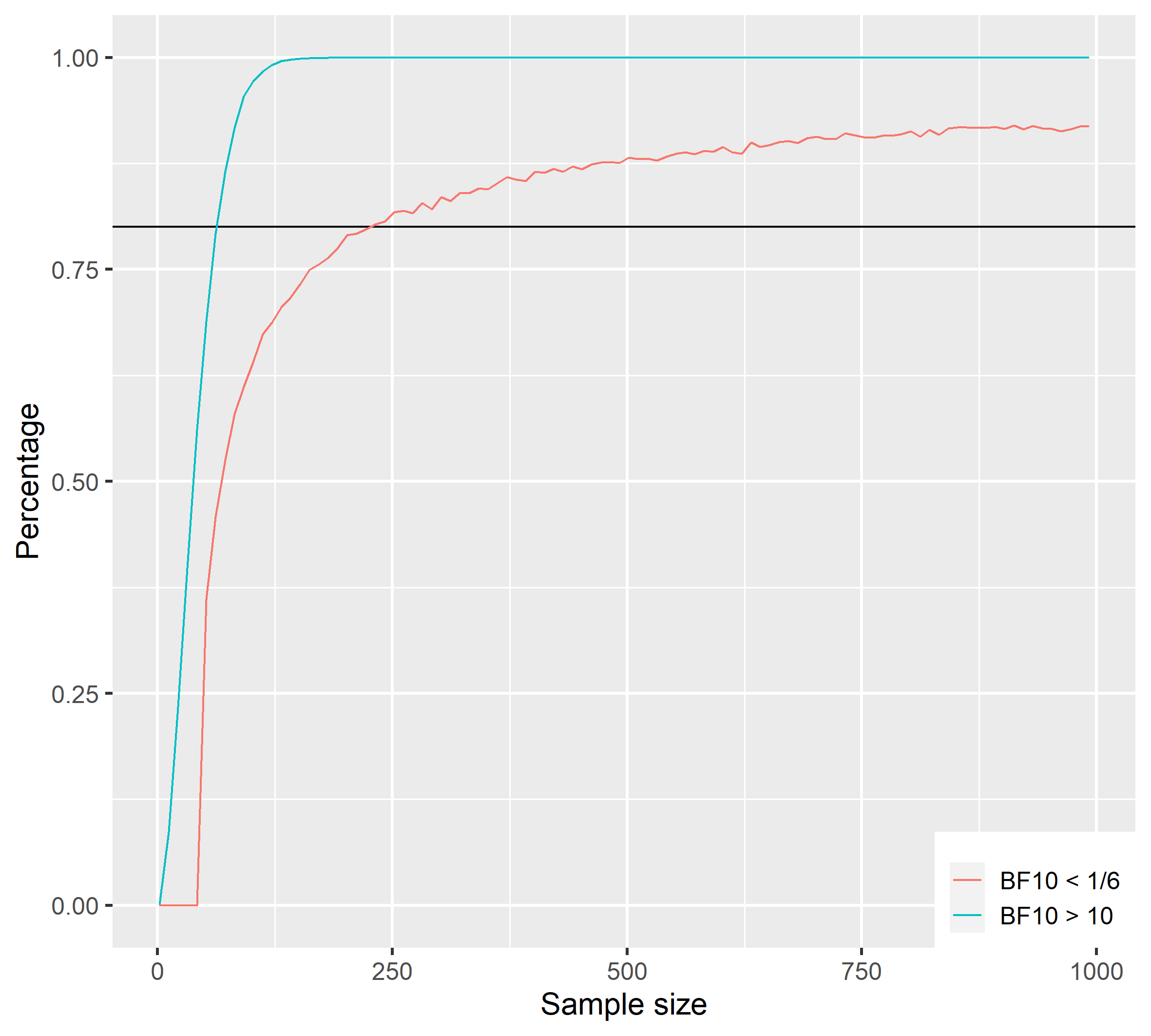
Above you can see the results of a traditional fixed sample size design analysis. This analysis is based on a Bayesian one-sample t-test and shows the percentage of surpassing the criteria as a function of the sample size. The blue line shows the percentage for $BF_{10}$ over 10 for a true medium effect size, while the red line shows a $BF_{10}$ below 1/6 for a true null effect size. I chose this asymmetric cut-off because it is much more difficult to get strong evidence for the point $H_0$ than it is for the $H_1$. Actually, to reach high percentage values like 95 % (as some journals require), we would need a sample size that is much larger than this. By the way, this simulation like on the all in this post was based on 10,000 iterations. If we plan for true effect size of 0.5, the necessary sample size is 72, while it is 232 if the true effect size is 0.0. Collecting a sample size that is that large for one experiment is quite impossible for a basic science experiment in my field (cognitive neuroscience) if it is not run online. Also remember that this is a one-sample t-test with two inpendent samples the necessary sample size would be even larger.
The good thing though is that there is a way to reliably produce strong evidence with samples that are (on average) much smaller: Sequential Bayesian Designs. In a sequential design we essentially keep on collecting data until reach the one of the pre-specified evidence criteria for instance a $BF_{10} > 10$ or $BF_{10} < 1/6$. Below you see an piece of code that can run this kind of simulation in simple a loop.
|
|
In this example we start with a sample size of 10 and then keep adding 5
more data points until we either reach crit1 or crit2. The true
effect size here is 0.0. This simulation of 100 iterations is
illustrated in this animation highlighting the sequential nature of the
data collection. Note that the x-axis is the sample size. Each
individual line represents one run in this simulation.
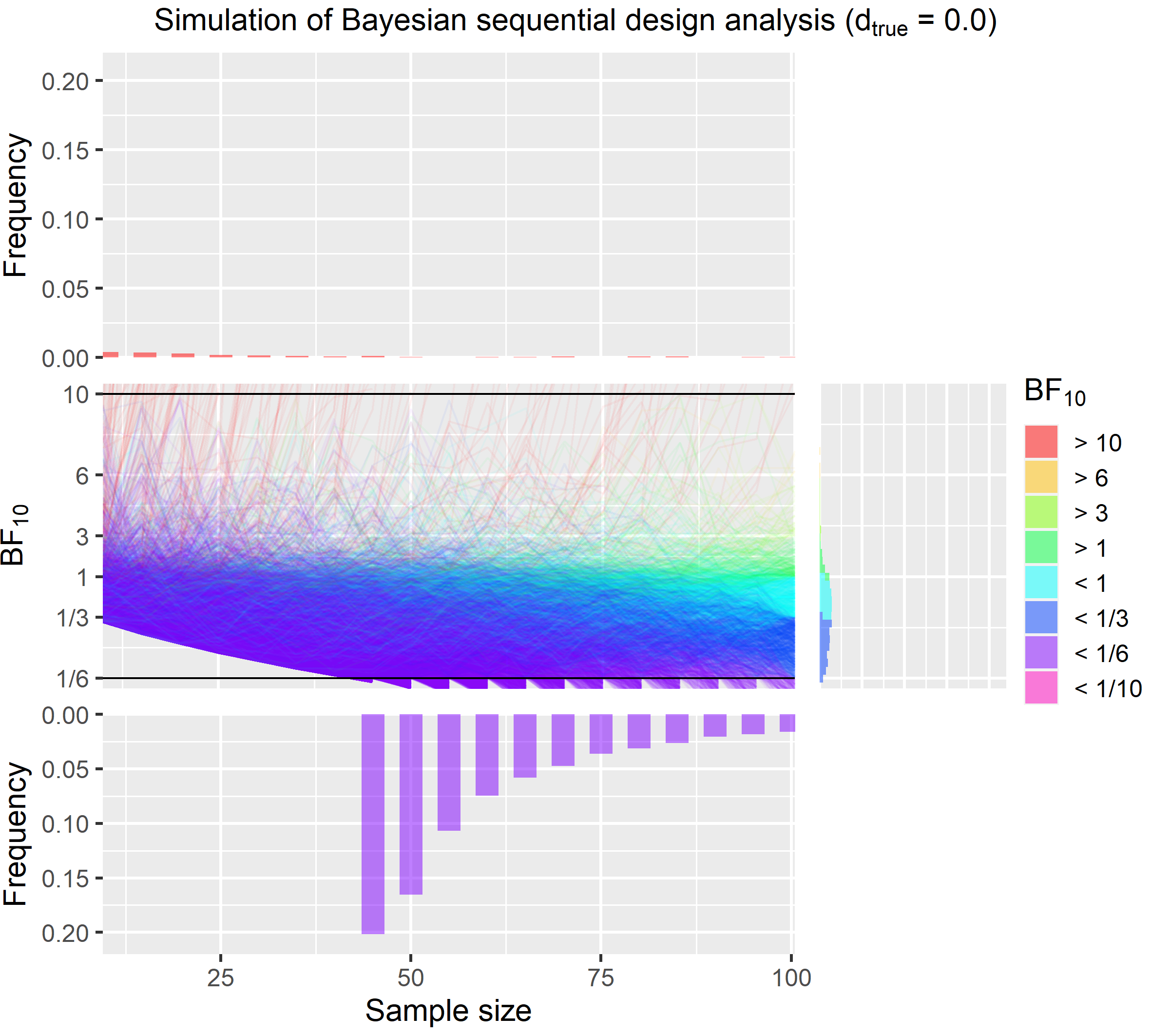
A full simulation of 10,000 iteration is shown in the figure below. The true effect size here is 0.0.
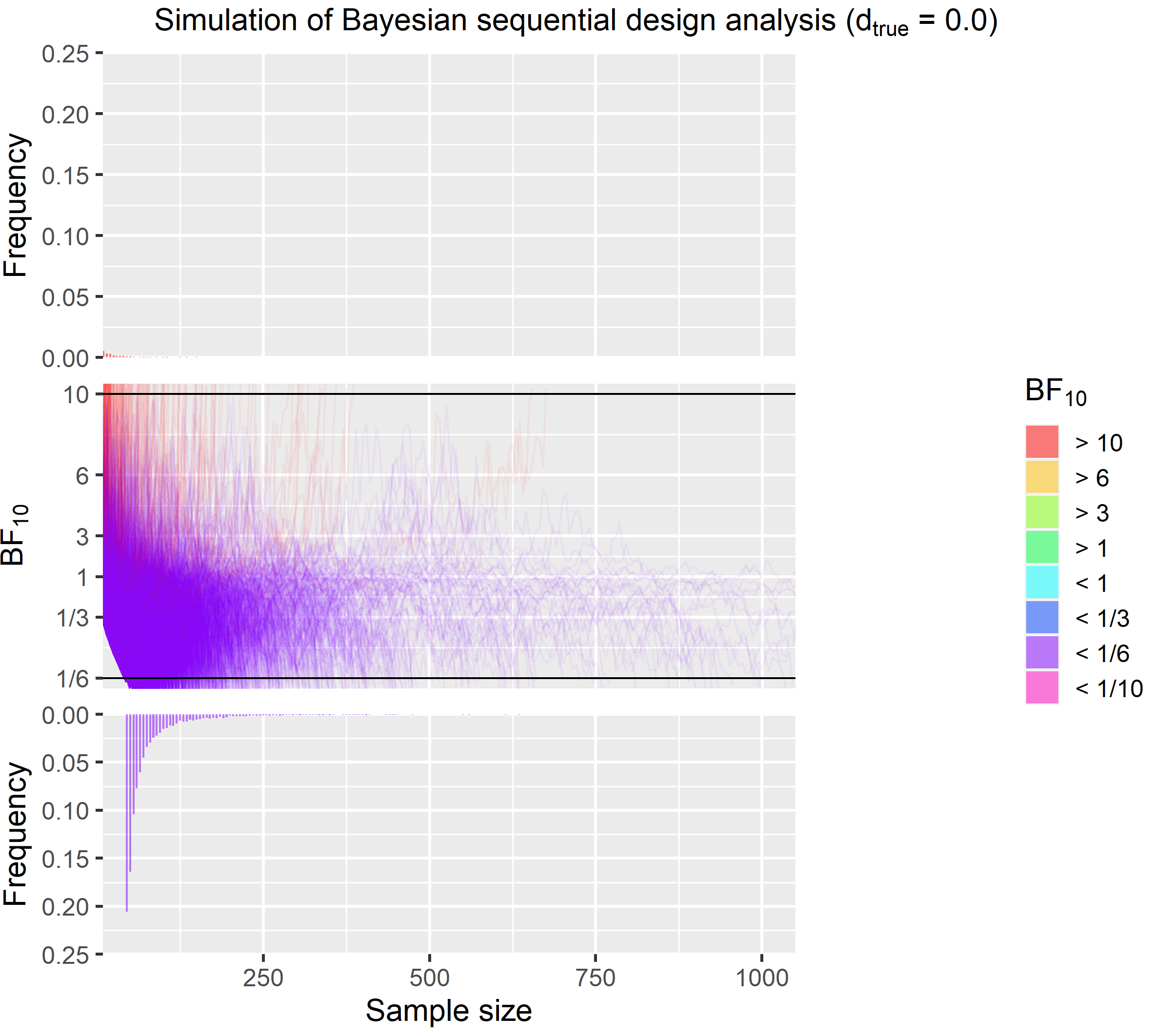
Here is a quick explanation of that this figure shows. Like in the animation, each individual line in the middle part of the figure represents one iteration of this simulation. The lines are colour coded based on the final BF (red = $BF_{10} > 10$, purple = $BF_{10} < 1/6$). At the top and the bottom, you see histograms showing how many BF were above and below the criteria for each sample size. Two things are apparent at the first glance. First, there is very little misleading evidence. Misleading evidence for this simulation means $BF_{10} > 10$. The red lines in the middle and the barely perceptible red bars in the top histogram visualise this. Second, most simulations end well before the 232 that are need to get a $BF_{10} < 1/6$ in 80 % of the times as in the traditional design but we also see that in some cases data collection goes well beyond 500 data points. In fact this figure is capped at 1000 for illustration. The highest sample size was actually 2765 and 10 were above 1000. However over average, we can stop data collection with sample size of only 83, which is much lower than the need in the traditional approach. For further illustration, I also present a simulation were we have true medium effect size.
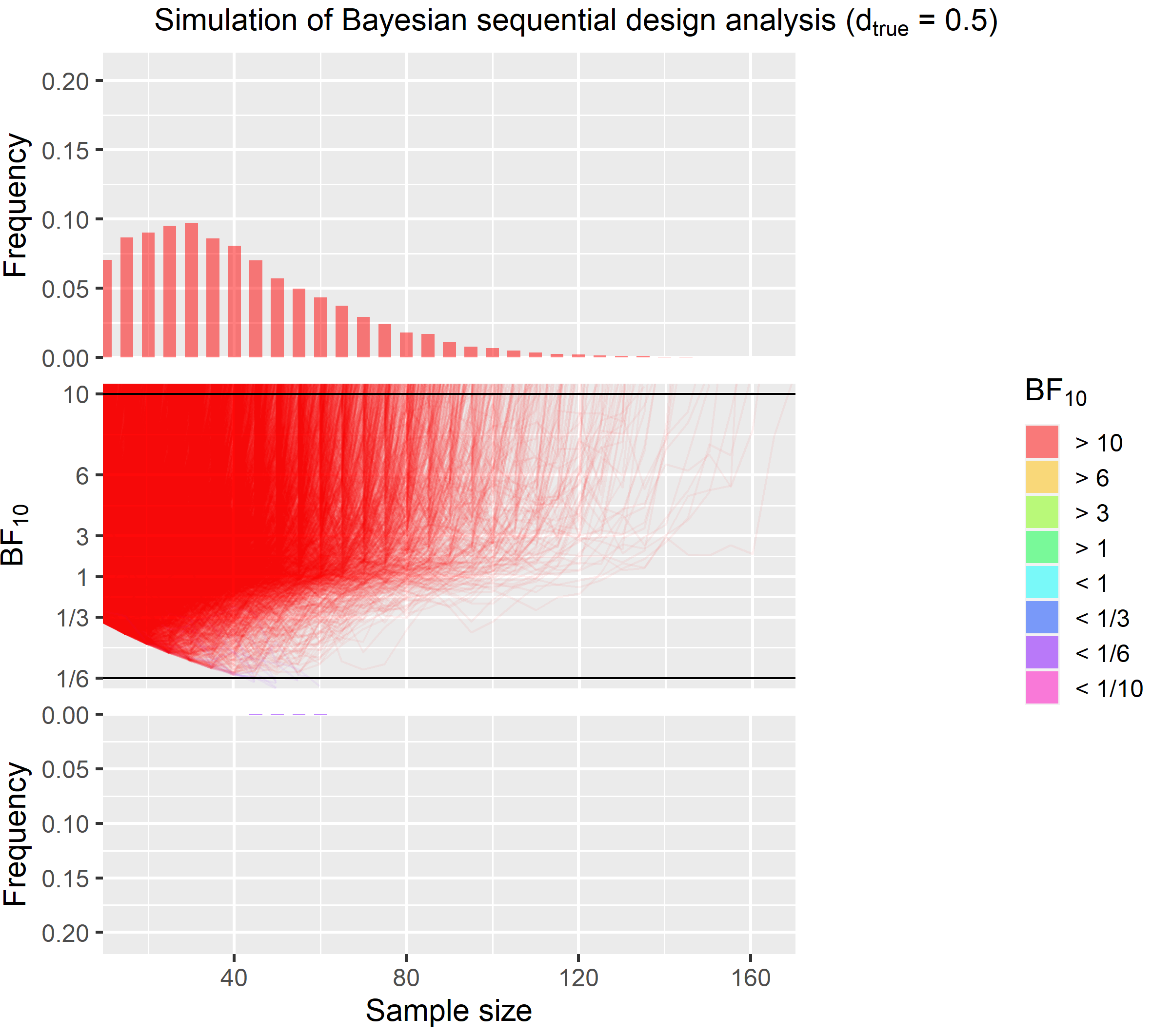
This figure also clearly shows that most runs end much earlier than the 72 from the fixed sample size design. The highest sample size for this effect size is 170.
Now, to the most interesting part that is comparing the traditional fixed sample size design and the sequential design directly. In the table below, you see the costs for an 1-hour long online experiment on prolific (£ 8.4) and an 1-hour long fMRI experiment (full economic costs of £ 550).
| Effect size | Necessary sample size | Misleading evidence in % | £ for online experiment | £ for fMRI experiment |
|---|---|---|---|---|
| 0.5 | 72 | 0.0003 | 605 | 39600 |
| 0.0 | 232 | 0.0011 | 1949 | 127600 |
Based on the results, we would need to spend a lot of money for each experiment. In the worst case scenario, where you plan to provide evidence for a null effect in fMRI experiment, you would have to spend £ 127600 it’s less if you plan for a medium effect size but the problem is often we don’t really have good estimate of the effect size. If we did, we might not even run the experiment. Johan Carlin recently gave a talk where he among other things discussed the problem of biased effect size estimates that lead to low power. His talk can be found here.
| Effect size | Average sample size | Maximal sample size | Misleading evidence in % | £ for online experiment | £ for fMRI experiment |
|---|---|---|---|---|---|
| 0.5 | 41 | 170 | 0.13 | 344 | 22550 |
| 0.0 | 83 | 2765 | 2.95 | 697 | 45650 |
With a true sequential design we don’t have this problem at all. Regardless of the true effect size we produce strong evidence and this on average much cheaper than with a fixed sample design. The average cost for an fMRI experiment for instance is only £ 45650. This is only 36 % of the cost that we’d have to play for a traditional design. At the same time, it needs to be acknowledged that the misleading evidence rates in much higher in sequential designs are much higher but still very low. For instance, for null effect in this simulation it is 2.95 %. If misleading evidence rates are of concerns then one thing that can be done is to increase the minimal sample size and the number of data points added in each batch. The effect of doing this is illustrated further below.
A much bigger problem is that while the average sample size is much lower, sometimes we’re unlucky and we haven’t reached a stopping criterion even after 1000 data points. For a PhD student running an fMRI experiment, this is just not feasible. Despite what 2 Unlimited wants us to believe, practically there is often a limit that can be based on money, available participants or time constraints. One way to protect oneself against collecting extremely large samples is to set an upper limit and to accept that in rare and extreme cases we might stop despite note having reached a criterion and ending with inconclusive evidence. Something that can also happen in a fixed sample size design. In the following, I will present simulations where data collection is stopped after collecting 100 data points regardless of whether an evidence criterion is reached. The additional histogram on the right side illustrates the distribution of $BF_{10}$ when stopped at 100.
| Effect size | Average sample size | Strong evidence in % | Misleading evidence in % | Insufficient evidence in % |
|---|---|---|---|---|
| 0.5 | 39 | 98.05 | 0.12 | 1.83 |
| 0.0 | 58 | 80.25 | 2.31 | 17.44 |
Stopping at 100 data points protects against having to collect extremely large samples but this approach still produces solid evidence in most cases even is the true effect is zero.
Take home message
It is important to find the right parameters for the specific situation that will lead to the most efficient data collection. Several factors influence the performance of Bayesian Sequential Designs. Those are
- minimum sample size influences the rate of misleading evidence,
- batch size (i.e. after how many new data points we check evidence),
- choice priors and likelihood functions (If you want evidence for $H_0$, there are better choices for this type of data. See my previous post on this issue) and
- directed vs. undirected hypothesis.
To get some idea how the parameters affect the performance of the sequential designs I’ve compiled a summary table of a couple of simulation that I ran for this talk. All simulations have the same effect sizes and the same number of iterations (10,000).
| Design | Direction | Minimal N | Batch size | Maximal N | Effect size | BF > crit % | Sample size | Misleading evidence % | £ online epxeriment | £ fMRI experiment |
|---|---|---|---|---|---|---|---|---|---|---|
| Fixed n | 2-sided | NA | NA | NA | 0.5 | 80.00 | 72 | 0.0003 | 605 | 39600 |
| Fixed n | 2-sided | NA | NA | NA | 0.0 | 80.00 | 232 | 0.0011 | 1949 | 127600 |
| Fixed n | 1-sided | NA | NA | NA | 0.5 | 80.00 | 62 | 0.0000 | 521 | 34100 |
| Fixed n | 1-sided | NA | NA | NA | 0.0 | 80.00 | 232 | 0.0026 | 1949 | 127600 |
| Sequential | 2-sided | 10 | 5 | NA | 0.5 | 100.00 | 41 | 0.1300 | 344 | 22550 |
| Sequential | 2-sided | 10 | 5 | NA | 0.0 | 100.00 | 83 | 2.9500 | 697 | 45650 |
| Sequential | 1-sided | 10 | 5 | NA | 0.5 | 100.00 | 34 | 1.1400 | 286 | 18700 |
| Sequential | 1-sided | 10 | 5 | NA | 0.0 | 100.00 | 62 | 3.3700 | 521 | 34100 |
| Sequential | 2-sided | 10 | 5 | 100 | 0.5 | 98.05 | 39 | 0.1200 | 328 | 21450 |
| Sequential | 2-sided | 10 | 5 | 100 | 0.0 | 80.25 | 58 | 2.3100 | 674 | 44138 |
| Sequential | 2-sided | 10 | 1 | 100 | 0.5 | 98.19 | 35 | 0.1800 | 294 | 19250 |
| Sequential | 2-sided | 10 | 1 | 100 | 0.0 | 82.08 | 55 | 3.6900 | 689 | 45144 |
| Sequential | 2-sided | 2 | 5 | 100 | 0.5 | 98.05 | 39 | 0.2500 | 328 | 21450 |
| Sequential | 2-sided | 2 | 5 | 100 | 0.0 | 79.27 | 59 | 2.9500 | 666 | 43599 |
Surprising sequential designs seem to be actually realtively robust. Note that the estimation of the misleading evidence rates also seems to be a bit noisy (despite running 10,000 iterations). For the scope of my talk I haven’t ran more simulations but it can be expected to find clearer results eith more extreme cases are compared.
All in all, I hope that I could show that sequential designs perform well regardless of the sampling plan and are in most cases to fixed sample size designs. I think as institutions and individuals dealing with money from tax payers we should try to work efficiently. Therefore, we should collect only as much data as we need. Obviously this is even more important if our work (potentially) causes harm as in animal experiments or work with patients.
References
Schönbrodt, F. D., & Wagenmakers, E.-J. (2018). Bayes factor design analysis: Planning for compelling evidence. Psychonomic Bulletin & Review, 25(1), 128–142. https://doi.org/10.3758/s13423-017-1230-y
Code
The data and the source code can be found here. The .Rmd file used to generated the code can be found here.